Lesson 10: Single Variable Modeling

Objectives

Given observed data, determine the most appropriate function type to model it.
Given data and a proposed model type, approximate the parameters by hand.
In R, use fitModel() to obtain the best-fit model of the most appropriate type.
Describe how collecting additional data can change how the model fits or which model type is most appropriate.
Describe the two primary reasons for modeling data: inference and prediction.
Define extrapolation, and which input values a model can be expected to give reasonable outputs for.

Testing Tips

Skim the whole quiz first. A first pass shows which questions will take longest.
Keep moving. Leave a question that stalls and come back to it at the end.
Read the instructions before the quiz: Math 141 Quiz 1 Instructions (Teams).
Scope: every objective through Lesson 10 is on the quiz.

Function Family Explorer Open full screen

1. Choosing the Model Family

Objective. Given observed data, determine the most appropriate function type to model it.

Model families.

Family	Model form	Identifying feature	Plot in R
Linear	$y = mx + b$	standard plot linear	`plotPoints(y ~ x)`
Exponential	$y = Ce^{k(x - h)}$	semi-log plot linear	`plotPoints(log(y) ~ x)`
Power	$y = Cx^{k}$	log-log plot linear	`plotPoints(log(y) ~ log(x))`
Sine	$y = A\sin\!\left(\frac{2\pi}{P}(x - h)\right) + v$	oscillates and repeats	`plotPoints(y ~ x)`
Sigmoid	$y = A\cdot\text{\rcmd{pnorm}}(x, m, s) + v$	levels off at both ends	`plotPoints(y ~ x)`

Choosing from the plots.

Graph the standard plot. If it is linear, then a linear model is reasonable.
If the standard plot oscillates and repeats, then a sine model is reasonable.
If the standard plot levels off at both ends, then a sigmoid model is reasonable. A sigmoid model is also reasonable when the plot levels off at one end and the situation supplies the level at the other, as for TwitterUsers3 on the Lesson 9 sheet.
If the standard plot rises or falls along a curve, graph the semi-log plot and the log-log plot. If the semi-log plot is linear, an exponential model is reasonable. If the log-log plot is linear, a power model is reasonable.
If more than one plot is close to linear, then the most appropriate family is the one whose plot keeps one slope from end to end, with no bend. When neither plot bends, both families are reasonable, as in Example 2.

Axis labels. Check the axis labels before judging the shape, because the standard, semi-log, and log-log plots look alike in R apart from their labels. A straight plot with $\ln(y)$ on the vertical axis and $x$ on the horizontal axis is a linear semi-log plot.

Example 1

The NASDAQQuarterly dataset records the closing NASDAQ value Close in dollars at the end of each quarter. A Quarter of 1 is March 1938, and a Quarter of 308 is December 2014. Determine the most appropriate function type to model Close as a function of Quarter.

ShowHide solution

Graph the standard, semi-log, and log-log plots:

plotPoints(Close ~ Quarter, data = NASDAQQuarterly)
plotPoints(log(Close) ~ Quarter, data = NASDAQQuarterly)
plotPoints(log(Close) ~ log(Quarter), data = NASDAQQuarterly)

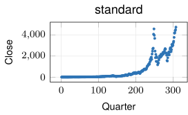
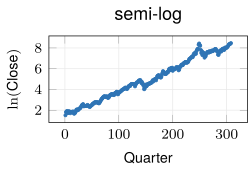
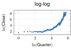
R labels the vertical axis of the last two plots log(Close), its spelling of $\ln(\text{Close})$ . The standard plot curves upward: the closing value stays below 500 until Quarter 215 and reaches 4736.05 at Quarter 308. The semi-log plot follows one straight trend from Quarter 1 to Quarter 308, apart from a bump around Quarter 249, where the closing value peaks at 4572.83 and then falls to 1335.51 by Quarter 260. The log-log plot bends upward across the whole record. An exponential model is the most appropriate, because the semi-log plot is the one with a straight trend.

Example 2

The NaturalGasConsumption dataset records United States natural gas consumption CubicFeet in millions of cubic feet for each Year from 1950 to 1970. Determine every function type that is a reasonable model of CubicFeet as a function of Year.

ShowHide solution

Graph the standard, semi-log, and log-log plots:

plotPoints(CubicFeet ~ Year, data = NaturalGasConsumption)
plotPoints(log(CubicFeet) ~ Year, data = NaturalGasConsumption)
plotPoints(log(CubicFeet) ~ log(Year), data = NaturalGasConsumption)

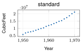
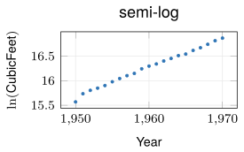
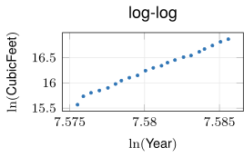
The standard plot curves upward. The semi-log and log-log plots both run straight from 1950 to 1970 with no bend, and they look alike, because $\ln(\text{Year})$ runs only from 7.5756 to 7.5858. Over an input interval that narrow and that far from 0, $\ln(x)$ is nearly linear in $x$ . An exponential model and a power model are both reasonable, because neither logged plot bends.

Next: 2. Approximating the Parameters by Hand Lesson map

2. Approximating the Parameters by Hand

Objective. Given data and a proposed model type, approximate the parameters by hand.

By-hand estimates.

Linear model. For $y = mx + b$ (Lesson 4 sheet, section 2), take $m$ and $b$ from the first data point $(x_1, y_1)$ and the last $(x_2, y_2)$ :

m = \frac{y_2 - y_1}{x_2 - x_1}, \qquad b = y_1 - m x_1.

Exponential model. For $y = Ce^{k(x - h)}$ (Lesson 5 sheet, section 2, and Lesson 6 sheet, sections 2 and 3), set $h = x_1$ , the first input. The constant $C$ is the output at $x = h$ , which makes $C = y_1$ . When $h = 0$ , the constant $C$ is the vertical intercept. The rate $k$ is the slope of the semi-log line through the first and last data points:

k = \frac{\ln(y_2) - \ln(y_1)}{x_2 - x_1}.

Power model. For $y = Cx^{k}$ (Lesson 7 sheet, section 3), take $k$ and $\ln(C)$ from the log-log line through the first and last data points:

k = \frac{\ln(y_2) - \ln(y_1)}{\ln(x_2) - \ln(x_1)}, \qquad \ln(C) = \ln(y_1) - k\ln(x_1), \qquad C = e^{\ln(C)}.

Sine model. For $y = A\sin\!\left(\frac{2\pi}{P}(x - h)\right) + v$ (Lesson 8 sheet, section 3), take $v$ and $A$ from a top level $y_{\max}$ and a bottom level $y_{\min}$ :

v = \frac{y_{\max} + y_{\min}}{2}, \qquad A = \frac{y_{\max} - y_{\min}}{2}.

The period $P$ is the input distance from one peak to the next. The horizontal shift $h$ is the first input where the data cross $y = v$ while increasing.

Sigmoid model. For $y = A\cdot\text{\rcmd{pnorm}}(x, m, s) + v$ (Lesson 9 sheet, section 4), take $v$ and $A$ from the levels $L$ on the left and $R$ on the right:

v = L, \qquad A = R - L.

The mean $m$ is the input where the data pass the halfway output $v + \frac{A}{2}$ . Let $x_{5/6}$ be the input where the data pass the five-sixths level $v + \frac{5A}{6}$ . The spread is $s = x_{5/6} - m$ .

Example 3

The TwitterUsers1 dataset records Twitter users Users in millions for eight quarters. The variable Year counts years since 2000. The first data point is $(12, 117)$ , and the last is $(13.75, 231.7)$ . Approximate the parameters of a linear model by hand.

ShowHide solution

The line through the first and last data points has

m = \frac{y_2 - y_1}{x_2 - x_1}, \qquad b = y_1 - m x_1.

Substituting $(x_1, y_1) = (12, 117)$ and $(x_2, y_2) = (13.75, 231.7)$ gives

m = \frac{231.7 - 117}{13.75 - 12} = \frac{114.7}{1.75} \approx 65.543, \qquad b = 117 - \frac{114.7}{1.75}(12) \approx -669.514.

The by-hand model is $\text{Users} = 65.543\,\text{Year} - 669.514$ .

Example 4

The NaturalGasConsumption dataset records 5,766,542 million cubic feet in 1950, its first year, and 21,139,386 in 1970, its last. Approximate by hand the parameters of the exponential model

\text{CubicFeet} = Ce^{k(\text{Year} - h)}.

ShowHide solution

Take $h = 1950$ , the first input. Then $C = 5{,}766{,}542$ , the output at $\text{Year} = h$ . The slope of the semi-log line through the first and last data points is $k$ :

k = \frac{\ln(y_2) - \ln(y_1)}{x_2 - x_1} = \frac{\ln(21{,}139{,}386) - \ln(5{,}766{,}542)}{1970 - 1950} \approx 0.064953.

The by-hand model is

\text{CubicFeet} = 5{,}766{,}542\,e^{0.064953(\text{Year} - 1950)}.

Example 5

The FiddlerCrabs dataset records the body size BodySize and the palm length PalmLength of growing male fiddler crabs, both in millimeters. The smallest crab has $\text{BodySize} = 3.43$ and $\text{PalmLength} = 1.07$ . The largest has $\text{BodySize} = 16.18$ and $\text{PalmLength} = 11.66$ . Approximate by hand the parameters of the power model

\text{PalmLength} = C\cdot\text{BodySize}^{k}.

ShowHide solution

The log-log line through the data points of the smallest and largest crabs has slope $k$ and intercept $\ln(C)$ :

k = \frac{\ln(11.66) - \ln(1.07)}{\ln(16.18) - \ln(3.43)}, \qquad \ln(C) = \ln(1.07) - k\ln(3.43).

R computes both values:

k = (log(11.66) - log(1.07))/(log(16.18) - log(3.43))
lnC = log(1.07) - k*log(3.43)
k
exp(lnC)

The last two lines print [1] 1.539764 and [1] 0.1603826. The by-hand model is

\text{PalmLength} = 0.160\,\text{BodySize}^{1.540}.

Example 6

The HenWeight dataset records the mean Weight of hens in grams at ages Day 0 to 170. Approximate the parameters of a sigmoid model by hand.

ShowHide solution

The data start from the hatching weight, about $L = 37$ , and levels off near $R = 1720$ :

v = L = 37, \qquad A = R - L = 1720 - 37 = 1683.

The halfway output $v + \frac{A}{2} = 37 + \frac{1683}{2} = 878.5$ falls between Day 71, at 832.57, and Day 85, at 1009.48. Join those two data points with a straight line. On it, $m$ lies the same fraction of the way from Day 71 to Day 85 as 878.5 lies from 832.57 to 1009.48:

m = 71 + \frac{878.5 - 832.57}{1009.48 - 832.57}(85 - 71) \approx 74.6.

The five-sixths level $v + \frac{5A}{6} = 37 + \frac{5(1683)}{6} = 1439.5$ lies just below the Day 113 weight, 1440.18. The five-sixths crossing is $x_{5/6} \approx 113$ , and the spread is

s = x_{5/6} - m \approx 113 - 74.6 = 38.4.

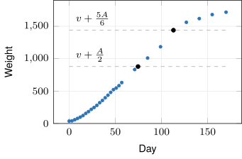
In the figure, the dashed lines are the halfway output 878.5 and the five-sixths level 1439.5. The black points are $(m, 878.5) = (74.6, 878.5)$ and $(x_{5/6}, 1439.5) = (113, 1439.5)$ , where the data pass those two levels. The by-hand model is

\text{Weight} = 1683\cdot\text{\rcmd{pnorm}}(\text{Day}, 74.6, 38.4) + 37.

Next: 3. Obtaining the Best Fit in R Lesson map

3. Obtaining the Best Fit in R

Objective. In R, use fitModel() to obtain the best-fit model of the most appropriate type.

Linear, exponential, and power models are fitted as a line on the plot that straightens them: the standard, semi-log, or log-log plot. Sine and sigmoid models are fitted on the standard plot. Their fits need starting values, start=, taken from the by-hand estimates of section 2.

In each call below, y stands for the output’s name, x for the input’s name, and D for the dataset’s name. Spell each name as in the dataset.

fitModel() by family.

Linear model

fitModel(y ~ m*x + b, data = D)

Exponential model

fitModel(log(y) ~ m*(x - h) + b, data = D)

Type the number for $h$ , as in m*(Year - 1950). Then $k = m$ and $C = e^{b}$ .

Power model

fitModel(log(y) ~ m*log(x) + b, data = D)

Then $k = m$ and $C = e^{b}$ .

Sine model

fitModel(y ~ A*sin(2*pi/P*(x - h)) + v, data = D,

start = list(A = ..., P = ..., h = ..., v = ...))

Sigmoid model

fitModel(y ~ A*pnorm(x, m, s) + v, data = D,

start = list(A = ..., m = ..., s = ..., v = ...))

Typed-in data. For data typed in as vectors with c(), leave data = off the call (Lesson 4 sheet, section 3).

Outputs of a log fit. A model fitted to log(y) returns outputs in the data’s own units. Applying exp() to those outputs is a mistake.

Singular gradient error. The function fitModel() stops with this error when a sine or sigmoid fit has no start=. It also stops with this error when the formula has a letter where a number belongs, such as h in an exponential fit.

> fitModel(log(CubicFeet) ~ m*(Year - h) + b, data = NaturalGasConsumption)
Error in nlsModel(formula, mf, start, wts, scaleOffset = scOff, nDcentral = nDcntr) :
  singular gradient matrix at initial parameter estimates

Drawing the fit. The function fitModel() prints no warning when a fit is poor. Draw every fit on its data:

Plot the data with plotPoints().
Add the fitted model with plotFun(..., add = TRUE).
Check that the curve passes through the data across the whole input interval, with no stretch where the points sit all above or all below it.

Example 7

For the NaturalGasConsumption dataset of Example 2, use fitModel() to obtain the best-fit exponential model with $h = 1950$ , and graph it with the data.

ShowHide solution

Fit the semi-log line with $h = 1950$ and print its slope and intercept:

gasExp = fitModel(log(CubicFeet) ~ m*(Year - 1950) + b,
data = NaturalGasConsumption)
coef(gasExp)

The last line prints

m b
0.06052149 15.66248660

Then

k = m \approx 0.060521, \qquad C = e^{b} = e^{15.66248660} \approx 6{,}340{,}617.

The best-fit model is

\text{CubicFeet} = 6{,}340{,}617\,e^{0.060521(\text{Year} - 1950)}.

Graph the fitted model function with the data:

plotPoints(CubicFeet ~ Year, data = NaturalGasConsumption)
plotFun(gasExp(Year) ~ Year, add = TRUE, col = "red")

The curve stays within 10 percent of every recorded value from 1950 to 1970.

Example 8

The table gives the cumulative worldwide sales of the Nintendo Switch in millions of units, from the NintendoSwitch dataset.

Year	2017	2018	2019	2020	2021	2022	2023	2024
Sales	13.12	29.46	48.82	76.83	100.96	120.01	136.41	142.37

Type the table into R, and use fitModel() to obtain the best-fit sigmoid model.

ShowHide solution

Estimate the four parameters by hand, then use them as starting values for fitModel(). Cumulative sales start from $L = 0$ before the 2017 launch and level off near $R = 145$ , which gives

v = L = 0, \qquad A = R - L = 145 - 0 = 145.

The halfway output $v + \frac{A}{2} = 0 + \frac{145}{2} = 72.5$ falls between 2019, at 48.82, and 2020, at 76.83. Interpolate between those two data points as in Example 6:

m = 2019 + \frac{72.5 - 48.82}{76.83 - 48.82}(2020 - 2019) \approx 2019.8.

The five-sixths level $v + \frac{5A}{6} = 0 + \frac{5(145)}{6} \approx 120.833$ falls between 2022, at 120.01, and 2023, at 136.41. Interpolating the same way gives

x_{5/6} = 2022 + \frac{120.833 - 120.01}{136.41 - 120.01}(2023 - 2022) \approx 2022.1.

The spread is

s = x_{5/6} - m = 2022.1 - 2019.8 = 2.3.

Type in the table and fit from these starting values:

Year = c(2017:2024)
Sales = c(13.12, 29.46, 48.82, 76.83, 100.96, 120.01, 136.41, 142.37)
ns = fitModel(Sales ~ A*pnorm(Year, m, s) + v,
start = list(A = 145, m = 2019.8, s = 2.3, v = 0))
coef(ns)
plotPoints(Sales ~ Year)
plotFun(ns(Year) ~ Year, add = TRUE, col = "red")

The coef() line prints

A m s v
150.833139 2019.897051 2.302102 -2.339220

The best-fit model is

\text{Sales} = 150.833\cdot\text{\rcmd{pnorm}}(\text{Year}, 2019.897, 2.302) - 2.339.

Next: 4. Additional Data and the Model Choice Lesson map

4. Additional Data and the Model Choice

Objective. Describe how collecting additional data can change how the model fits or which model type is most appropriate.

Additional data can change the most appropriate family. Over a short enough input interval, every smooth curve looks close to linear, and a short record may show only that nearly straight stretch. The bends of the curve appear as the record grows, as in Example 9.

Additional data can also keep the family and change the fitted parameters. A short record leaves a parameter poorly determined, and more data can move it a long way, as in Example 10.

Example 9

The TwitterUsers datasets record Twitter users Users in millions by quarter. The variable Year counts years since 2000.

The dataset TwitterUsers1 has eight quarters, Year 12 to 13.75.
The dataset TwitterUsers2 has those eight and the seven before them, from Year 10.25.
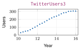
The dataset TwitterUsers3 has all fifteen and nine more, through Year 16.

Determine the most appropriate function type for each dataset. Then describe how the additional data changed the choice.

ShowHide solution

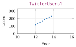
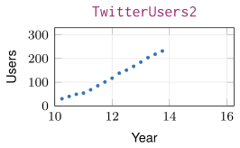
Linear model for TwitterUsers1. The eight readings are 117, 138, 151, 167, 185, 204, 218, and 231.7 million users, and they climb steadily. The slopes between successive points are 84, 52, 64, 72, 76, 56, and 54.8 million users per year, with no trend. Fit a line:

t1 = fitModel(Users ~ m*Year + b, data = TwitterUsers1)
coef(t1)

The last line prints

m b
65.70952 -669.54762

The best-fit line is $\text{Users} = 65.710\,\text{Year} - 669.548$ .

Power model for TwitterUsers2. The seven added quarters rise slowly, and the eight quarters of TwitterUsers1 rise faster. One line cannot follow both stretches. The semi-log plot bends downward, and the log-log plot is closer to linear:

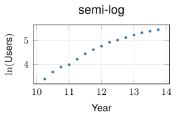
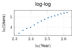
Graph both plots and fit the log-log line:

plotPoints(log(Users) ~ Year, data = TwitterUsers2)
plotPoints(log(Users) ~ log(Year), data = TwitterUsers2)
t2 = fitModel(log(Users) ~ m*log(Year) + b, data = TwitterUsers2)
coef(t2)

The last line prints

m b
6.979725 -12.686064

The best-fit power model is $\text{Users} = e^{-12.686}\,\text{Year}^{6.980}$ .

Sigmoid model for TwitterUsers3. The nine added quarters level off near 305 million users. The power model no longer fits, because a power model with $C > 0$ and a positive exponent rises without a ceiling, while a sigmoid model levels off. For starting values, users start from $v = 0$ and level off near 305, which gives $A = 305 - 0 = 305$ . The halfway output $0 + \frac{305}{2} = 152.5$ falls near Year 12.5, which gives $m = 12.5$ . The five-sixths level $0 + \frac{5(305)}{6} \approx 254.2$ falls near Year 14.25, and the spread is

s = 14.25 - 12.5 = 1.75.

Fit from these starting values:

t3 = fitModel(Users ~ A*pnorm(Year, m, s) + v, data = TwitterUsers3,
start = list(A = 305, m = 12.5, s = 1.75, v = 0))
coef(t3)

The last line prints

A m s v
325.967050 12.624146 1.870370 -3.973633

The best-fit sigmoid model is

\text{Users} = 325.967\cdot\text{\rcmd{pnorm}}(\text{Year}, 12.624, 1.870) - 3.974.

The most appropriate family changed twice, from linear to power to sigmoid, while the eight points of TwitterUsers1 stayed the same. They are the steep middle of the sigmoid, and only the quarters added on each side show its bends.

Example 10

The TemperaturesDanville dataset records the average maximum temperature in degrees Fahrenheit in Danville, Kentucky, at the start of each month, with Month 0 to 59 counting months from January 2006. Fit a sine model to the first 12 months alone (Month 0 to 11), then to all 60 months, from the same starting values. Compare the two periods, and compare each model’s output at Month 30 with the recorded 86 degrees.

ShowHide solution

Approximate the starting values by hand from the plot of all 60 months, drawn on the Lesson 8 sheet, section 2. A level of 88 through the typical peaks and one of 32 through the typical troughs give

v = \frac{88 + 32}{2} = 60, \qquad A = \frac{88 - 32}{2} = 28.

Temperature repeats each year, which gives $P = 12$ months. The data cross 60 while increasing between Month 2 (53.8) and Month 3 (69.3), and the midpoint of the two months gives $h = 2.5$ . Fit both models from these values, print their parameters, and evaluate each at 30:

year1 = TemperaturesDanville[TemperaturesDanville$Month <= 11, ]
fit1 = fitModel(Temperature ~ A*sin(2*pi/P*(Month - h)) + v, data = year1,
start = list(A = 28, P = 12, h = 2.5, v = 60))
fitAll = fitModel(Temperature ~ A*sin(2*pi/P*(Month - h)) + v,
data = TemperaturesDanville,
start = list(A = 28, P = 12, h = 2.5, v = 60))
coef(fit1)
coef(fitAll)
fit1(30)
fitAll(30)

The two coef() lines print

A P h v
18.835429 10.875087 3.330367 67.288006
A P h v
23.286833 11.982097 3.163625 65.358279

and the last two lines print [1] 72.84217 and [1] 88.59642. The one-year fit has period $P \approx 10.875$ months, short of the 12-month year. At Month 30 it gives about 72.842 degrees, which falls $86 - 72.842 = 13.158$ degrees below the recorded value. The five-year fit has $P \approx 11.982$ months. At Month 30 it gives about 88.596 degrees, which lies $88.596 - 86 = 2.596$ degrees above the recorded value. The family stayed the same. The four added years of data moved the period close to 12 months and the prediction close to the record.

Next: 5. Inference and Prediction Lesson map

5. Inference and Prediction

Objective. Describe the two primary reasons for modeling data: inference and prediction.

Definition 1 (Inference).

Inference is the use of a model’s fitted parameters to describe how the output variable depends on the input variable.

An inference question asks how the variables relate: whether the output grows or decays, at what rate, and on what cycle.

The model’s output at one chosen input, such as the gas consumption it gives for 1965.5, is not an inference, because it describes no relationship between the variables. The definition of inference uses the fitted parameters to describe how the output depends on the input.

Definition 2 (Prediction).

Prediction is the use of a model to estimate the output value at a chosen input, typically one the data does not record.

A prediction question asks for the output at a chosen input.

The 5,766,542 million cubic feet recorded for 1950 in NaturalGasConsumption is not a prediction, because it comes from the data’s own row. The definition of prediction requires a model to estimate the output.

Example 11

The best-fit exponential model for NaturalGasConsumption, 1950 to 1970, is

\text{CubicFeet} = 6{,}340{,}617\,e^{0.060521(\text{Year} - 1950)}.

Classify each question as inference or prediction, and answer it.

(a) Was natural gas consumption growing from 1950 to 1970, and at what rate?
(b) What consumption does the model give at Year 1965.5, halfway between the recorded years 1965 and 1966?

ShowHide solution

(a) The question is an inference, because by the definition of inference its answer comes from the fitted parameter $k$ , which describes how consumption depends on the year. Consumption was growing, because $k \approx 0.060521$ is positive. The growth rate was about 6 percent per year.

(b) The question is a prediction, because by the definition of prediction its answer is the model’s estimate of the output at a chosen input, here one the data do not record. Fit the model and evaluate it at 1965.5:

gasExp = fitModel(log(CubicFeet) ~ m*(Year - 1950) + b,
data = NaturalGasConsumption)
gasExp(1965.5)

The last line prints [1] 16200777: the model gives 16,200,777 million cubic feet at Year 1965.5.

Example 12

The best-fit sine model for all 60 months of TemperaturesDanville is

\text{Temperature} = 23.287\sin\!\left(\frac{2\pi}{11.982}(\text{Month} - 3.164)\right) + 65.358.

Classify each question as inference or prediction.

(a) How long is one cycle of Danville’s temperatures?
(b) What average maximum temperature does the model give for February 2024?
(c) By how many degrees do the summer peaks exceed the winter troughs?

ShowHide solution

(a) Inference, because the fitted period $P \approx 11.982$ months answers it.

(b) Prediction, because it asks for the model’s output at one input. With Month 0 in January 2006, February 2024 is Month $(2024 - 2006)(12) + 1 = 217$ , an extrapolation 158 months past the data.

Next: 6. Extrapolation and Reliable Input Values Lesson map

6. Extrapolation and Reliable Input Values

Objective. Define extrapolation, and which input values a model can be expected to give reasonable outputs for.

An interpolation is a prediction at an input that lies inside the input interval used to create the model.

Definition 3 (Extrapolation).

An extrapolation is a prediction at an input that lies outside the input interval used to create the model.

An extrapolation can be far off, because the data give no evidence about outputs at inputs outside the input interval used to create the model.

The prediction at Year 1965.5 in Example 11 is not an extrapolation, because 1965.5 lies inside the input interval 1950 to 1970 used to create the model. The definition requires an input outside that interval.

Reliable input values. A model can be expected to give reasonable outputs for inputs inside the input interval used to create it. The statement applies to a model that is reasonable for the data, as judged in section 1, and drawn on the data as in section 3.

A sine model that is reasonable for data from a repeating process, such as the seasons, also gives reasonable outputs a cycle past the data, because the process repeats.

Beside every extrapolated answer, state the input interval used to create the model, as in Example 14.

Example 13

The NASDAQQuarterly dataset records the closing NASDAQ value Close for Quarter 1 to 308. Fit the exponential model with $h = 0$ :

\text{Close} = Ce^{k\cdot\text{Quarter}}.

Evaluate the model at Quarter 220 and at Quarter 340, and state whether each evaluation is an interpolation or an extrapolation.

ShowHide solution

Fit the semi-log line with $h = 0$ and evaluate the model at each quarter:

nq = fitModel(log(Close) ~ m*Quarter + b, data = NASDAQQuarterly)
nq(220)
nq(340)

The last two lines print [1] 638.7816 and [1] 9602.522. The value 638.782 at Quarter 220 is an interpolation, because 220 lies inside the input interval 1 to 308 used to create the model. The recorded value in the data’s row for Quarter 220 is 676.95, and the model’s value falls 38.168 below it, about 5.6 percent of the recorded value. By the definition of extrapolation, the value 9602.522 at Quarter 340 is an extrapolation, because 340 lies outside the input interval 1 to 308 used to create the model.

Example 14

The most appropriate models for the TwitterUsers datasets of Example 9 are linear for TwitterUsers1 (Year 12 to 13.75), power for TwitterUsers2 (Year 10.25 to 13.75), and sigmoid for TwitterUsers3 (Year 10.25 to 16). Fit the three models, evaluate each at Year 15.5, and state whether each evaluation is an interpolation or an extrapolation. Compare each value with the 304 million users recorded at Year 15.5.

ShowHide solution

The sigmoid needs starting values from the TwitterUsers3 data. Users start from $v = 0$ and level off near 305, which gives $A = 305$ . The data pass the halfway output $0 + \frac{305}{2} = 152.5$ near Year 12.5 and the five-sixths level $0 + \frac{5(305)}{6} \approx 254.2$ near Year 14.25:

m = 12.5, \qquad s = 14.25 - 12.5 = 1.75.

Fit the three models and evaluate each at Year 15.5:

t1 = fitModel(Users ~ m*Year + b, data = TwitterUsers1)
t2 = fitModel(log(Users) ~ m*log(Year) + b, data = TwitterUsers2)
t3 = fitModel(Users ~ A*pnorm(Year, m, s) + v, data = TwitterUsers3,
start = list(A = 305, m = 12.5, s = 1.75, v = 0))
t1(15.5)
t2(15.5)
t3(15.5)

The last three lines print [1] 348.95, [1] 629.0712, and [1] 301.759.

Model	Input interval	At Year 15.5	Evaluation
Linear, `t1`	12 to 13.75	348.950	extrapolation
Power, `t2`	10.25 to 13.75	629.071	extrapolation
Sigmoid, `t3`	10.25 to 16	301.759	interpolation

The interpolation lands within 3 million users of the recorded 304. The two extrapolations miss by about 45 million and about 325 million.

Lesson map