Lesson 9: Modeling with Sigmoid Functions

Objectives

In R, use pnorm() to define sigmoid functions of the form y = A*pnorm(x,m,s) + v.
Describe how a parameterized sigmoid changes as each parameter is adjusted.
Given a plot of data, determine whether a sigmoid model is appropriate.
Given data exhibiting a sigmoidal relationship, approximate the parameters by hand.
In R, use fitModel() to obtain the best-fit sigmoid model.
Evaluate a sigmoid model at a given input and interpret the answer.

TwitterUsers3 Dataset

The dataset TwitterUsers3, in the MMAC package, records monthly active Twitter users by quarter. It has 24 rows. The variable Year counts years since 2000. A Year of 10.25 is the second quarter of 2010, and a Year of 16 is the first quarter of 2016. The variable Users runs from 30 to 307 million.

Sigmoid Landmarks Open full screen

1. Sigmoid Functions in R

Objective. In R, use pnorm() to define sigmoid functions of the form y = A*pnorm(x,m,s) + v.

The TwitterUsers3 data climb steeply and then level off near 305 million users.

Definition 1 (Sigmoid function).

A sigmoid function is a function whose graph has an elongated S shape: it approaches one horizontal asymptote on the left and a different one on the right, and changes steeply between them.

The exponential function $y = e^{x}$ is not a sigmoid function. It approaches the horizontal asymptote $y = 0$ on the left, but it grows without bound on the right, and the definition requires a second horizontal asymptote on the right.

The R function pnorm(x, m, s), with $s > 0$ , is an increasing sigmoid function of $x$ . Its horizontal asymptotes are $y = 0$ on the left and $y = 1$ on the right, and its output is $0.5$ at $x = m$ . The call pnorm(x) means pnorm(x, 0, 1).

Definition 2 (Sigmoid model).

A sigmoid model gives the output $y$ as a stretched and shifted pnorm:

y = A\cdot\text{\rcmd{pnorm}}(x, m, s) + v.

The four parameters are the amplitude $A$ , the mean $m$ , the spread $s$ , and the vertical shift $v$ . The amplitude is nonzero, $A \ne 0$ , and the spread is positive, $s > 0$ .

In R, the general form is written y = A*pnorm(x, m, s) + v.

The function $y = 3\cdot\text{\rcmd{pnorm}}(x, 2, 0) + 1$ is not a sigmoid model, because its spread is $s = 0$ , and the definition requires $s > 0$ . With a spread of 0, pnorm jumps from 0 straight to 1 at $x = 2$ , and the graph is two flat pieces with no S between them.

R template for a sigmoid function.

f = makeFun(A*pnorm(x, m, s) + v ~ x)
plotFun(f(x) ~ x, xlim = range(LOW, HIGH))

Replace A, m, s, v, LOW, and HIGH with numbers.

Example 1

Define the sigmoid function

f(x) = 6\cdot\text{\rcmd{pnorm}}(x, 4, 2) + 2

in R, plot it for $-2 \le x \le 10$ , and evaluate it at $x = 4$ and $x = 6$ .

ShowHide solution

By the definition of a sigmoid model, $f$ has $A = 6$ , $m = 4$ , $s = 2$ , and $v = 2$ . Put those numbers into the R template, plot $f$ , and evaluate it at each input:

f = makeFun(6*pnorm(x, 4, 2) + 2 ~ x)
plotFun(f(x) ~ x, xlim = range(-2, 10))
f(4)
f(6)

The last two lines print [1] 5 and [1] 7.048068: $f(4) = 5$ and $f(6) \approx 7.048$ . As a check, $\text{\rcmd{pnorm}}(4, 4, 2) = 0.5$ at the mean, and

f(4) = 6(0.5) + 2 = 5.

Example 2

Define in R the sigmoid model with amplitude $A = 60$ , mean $m = 5$ , spread $s = 1.5$ , and vertical shift $v = 20$ , and evaluate it at $x = 3$ and $x = 5$ .

ShowHide solution

Substitute the four parameters into the general form of a sigmoid model:

p(x) = 60\cdot\text{\rcmd{pnorm}}(x, 5, 1.5) + 20.

Define $p$ in R and evaluate it at each input:

p = makeFun(60*pnorm(x, 5, 1.5) + 20 ~ x)
p(3)
p(5)

The last two lines print [1] 25.47267 and [1] 50: $p(3) \approx 25.473$ and $p(5) = 50$ . The input $x = 3$ lies left of the mean $m = 5$ , and its output 25.473 lies below the output $p(5) = 50$ at the mean, as an increasing function requires.

Negative spread. The function pnorm with a negative third argument returns NaN, R’s mark for a value that is not a number. A formula with a negative number in place of the spread $s$ evaluates to NaN as well.

> pnorm(2, 0, -1)
[1] NaN
Warning message:
In pnorm(2, 0, -1) : NaNs produced

Next: 2. Effects of the Sigmoid Parameters Lesson map

2. Effects of the Sigmoid Parameters

Objective. Describe how a parameterized sigmoid changes as each parameter is adjusted.

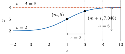
The curve $y = 6\cdot\text{\rcmd{pnorm}}(x, 4, 2) + 2$ of Example 1, with $A = 6$ , $m = 4$ , $s = 2$ , and $v = 2$ . The black points are $(m, f(m)) = (4, 5)$ and $(m + s, f(m + s)) \approx (6, 7.048)$ .

The vertical shift $v$ is the output the graph approaches as the inputs decrease without bound. The left horizontal asymptote is $y = v$ .

The amplitude $A$ is the output the graph approaches as the inputs increase without bound, minus $v$ . The right horizontal asymptote is $y = v + A$ .

The mean $m$ is the input at which the output is $v + \frac{A}{2}$ , halfway between the two horizontal asymptotes. The curve is steepest at $m$ .

The five-sixths level is the output five-sixths of the way from $v$ to $v + A$ , namely $v + \frac{5A}{6}$ .

The spread $s$ is the positive input distance from $m$ to the input where the output has covered pnorm(1) $\approx 0.8413$ of its change from $v$ to $v + A$ .

The fraction $\text{\rcmd{pnorm}}(1) \approx 0.8413$ is the output of pnorm one spread past the mean. The value of $\text{\rcmd{pnorm}}(x, m, s)$ depends only on how many spreads $x$ lies past $m$ , the number $\frac{x - m}{s}$ , and at $x = m + s$ that number is 1:

\text{\rcmd{pnorm}}(m + s, m, s) = \text{\rcmd{pnorm}}(1) \approx 0.8413.

The by-hand estimate of $s$ in section 4 uses the five-sixths level in place of the 0.8413 point, because 0.8413 is within 0.01 of $\frac{5}{6} \approx 0.8333$ .

The five-sixths level is also two thirds of the way from the halfway output to the level on the right, because two thirds of the remaining $\frac{A}{2}$ is $\frac{A}{3}$ , and $v + \frac{A}{2} + \frac{A}{3} = v + \frac{5A}{6}$ .

The sign of the amplitude $A$ determines whether a sigmoid model increases or decreases. Each graph shows a sigmoid model with its two horizontal asymptotes dashed.

Positive amplitude

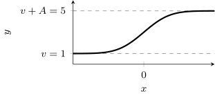
The model $y = 4\cdot\text{\rcmd{pnorm}}(x, 0, 1) + 1$ has $A = 4 > 0$ , and it increases from $v = 1$ to $v + A = 5$ . The number of people who have joined a network follows this shape as it climbs toward a ceiling.

Negative amplitude

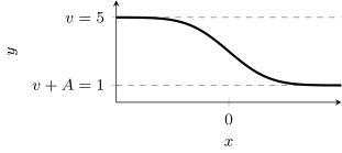
The model $y = -4\cdot\text{\rcmd{pnorm}}(x, 0, 1) + 5$ has $A = -4 < 0$ , and it decreases from $v = 5$ to $v + A = 1$ . The number of people not yet infected in an outbreak follows this shape as it falls toward a floor.

Parameters inside and outside pnorm. The mean $m$ and the spread $s$ sit inside pnorm and change the input. The mean slides the curve horizontally, and the spread stretches the curve horizontally. The amplitude $A$ and the vertical shift $v$ sit outside pnorm and change the output. The amplitude stretches the curve vertically, and a negative amplitude also flips it upside down. The vertical shift slides the curve vertically.

Amplitude and vertical shift in the sine and sigmoid models. The Lesson 8 sheet, section 1, defines $A$ and $v$ for the sine model, where $v$ is the middle level and $A$ is half the swing. In the sigmoid model, $v$ is the level on the left and $A$ is the whole change from the level on the left to the level on the right.

Example 3

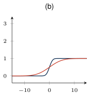
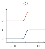
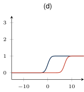
In each panel the dark blue curve is $\text{\rcmd{pnorm}}(x) = 1\cdot\text{\rcmd{pnorm}}(x, 0, 1) + 0$ . The red curve differs from $\text{\rcmd{pnorm}}(x)$ in exactly one parameter. Name the parameter that changed in each panel.

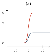
ShowHide solution

(a) The amplitude $A$ changed, because the level on the left held at 0 while the level on the right rose from 1 to 3.
(b) The spread $s$ changed, because both levels and the halfway output at $x = 0$ held while the rise spread over a much wider stretch of input.
(c) The vertical shift $v$ changed, because both levels rose by 2 together while the height of the rise held.
(d) The mean $m$ changed, because the whole curve slid right by 7 with the same height and the same steepness.

Example 4

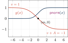
Describe how the graph of

g(x) = -2\cdot\text{\rcmd{pnorm}}(x, 0, 2) + 1

differs from the graph of $\text{\rcmd{pnorm}}(x)$ .

ShowHide solution

Three parameters differ from those of $\text{\rcmd{pnorm}}(x)$ , and the mean stays the same:

The vertical shift is $v = 1$ , which moves the level on the left from 0 up to 1.
Because the amplitude is $A = -2$ , the curve falls by 2, to $v + A = -1$ on the right.
Because the mean stays at $m = 0$ , the function $g$ passes its halfway output $1 + \frac{-2}{2} = 0$ at $x = 0$ .
The spread is $s = 2$ , which spreads the drop over twice the stretch of input that $\text{\rcmd{pnorm}}(x)$ takes to climb.

Next: 3. Recognizing Sigmoidal Data Lesson map

3. Recognizing Sigmoidal Data

Objective. Given a plot of data, determine whether a sigmoid model is appropriate.

Definition 3 (Sigmoidal data).

Sigmoidal data are data whose outputs stay near one level for small inputs, rise or fall steeply through a middle stretch, and level off at a different value for large inputs.

Data that stay near one level for small inputs and then climb faster and faster, as exponential data do, are not sigmoidal, because the definition requires the outputs to level off at a different value for large inputs.

Exponential and power data become lines on semi-log and log-log plots (Lessons 5 to 7). Neither plot straightens sigmoidal data across the whole record, because each logged plot still levels off where the data level off. Judge whether a sigmoid model is reasonable from the plot of the raw data.

Power curve and sigmoid at the left edge. A power curve with exponent between 0 and 1 also climbs and then slows. The two differ at the left edge, where the power curve is steepest at its first point and sigmoidal data start flat.

Limit from the situation. A sigmoid model is reasonable for a quantity with a limit, such as the number of people who can join a network or catch a disease. Without such a limit, a flattening in the record may be temporary. The situation can also supply a level that the record does not show, such as a count that starts from zero.

Example 5

Determine whether a sigmoid model is reasonable for TwitterUsers3.

ShowHide solution

Plot the data:

plotPoints(Users ~ Year,
data = TwitterUsers3)

The 24 quarterly readings climb steeply from Year 11 to about Year 14.5. The last five quarters stay between 288 and 307 million.

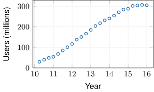
The definition of sigmoidal data asks for a level for small inputs, a steep middle stretch, and a different level for large inputs. The readings have the steep climb and the level on the right. The record has no level on the left, because it begins at 30 million users with the climb already under way. The situation supplies that missing level: Twitter started from zero users. With all three parts in place, a sigmoid model is reasonable.

Example 6

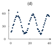
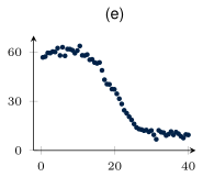
Each panel plots one dataset. Determine which panels a sigmoid model fits, and name the model family that fits each of the other panels.

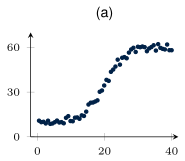
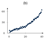
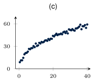
ShowHide solution

(a) Sigmoid, because the data run flat near 10, climb steeply around 20, and run flat near 60.
(b) Exponential, because the data climb more steeply at each step and never level off.
(c) Power, because the climb starts at the first point with no level on the left and slows across the whole record with no steep middle stretch.
(d) Sine, because the data rise, fall, and rise again.
(e) Sigmoid with a negative amplitude $A$ , because the data run flat near 60, drop steeply around 20, and run flat near 10.

Next: 4. By-Hand Estimates of the Parameters Lesson map

4. By-Hand Estimates of the Parameters

Objective. Given data exhibiting a sigmoidal relationship, approximate the parameters by hand.

Recipe for by-hand sigmoid estimates. Call the level the data settle to on the left $L$ , and the level they settle to on the right $R$ .

Take the vertical shift as the level on the left, $v = L$ .
Subtract to find the amplitude, $A = R - L$ .
Compute the halfway output $v + \frac{A}{2}$ , and take $m$ as the input where the data pass it.
Compute the five-sixths level $v + \frac{5A}{6}$ , estimate the input $x_1$ where the data pass it, and subtract, $s = x_1 - m$ .

Falling data. The same steps apply to data that fall from left to right. The level on the right is then below the level on the left, $R < L$ , and the amplitude $A = R - L$ is negative.

Missing level in the record. When the record never flattens at one end, the level at that end comes from the situation: the starting count, or the limit the count is heading for.

Spread as a difference. The spread $s$ is the distance from $m$ to $x_1$ , which step 4 finds by subtracting $m$ from the location $x_1$ .

Landmark check of an estimate. Mark four landmarks on the plot of the data, then sketch an S through them.

Draw a horizontal line at $y = v$ , the level on the left.
Draw a horizontal line at $y = v + A$ , the level on the right.
Mark the point $\left(m,\ v + \frac{A}{2}\right)$ at the halfway output.
Mark the point $\left(m + s,\ v + \frac{5A}{6}\right)$ at the five-sixths level.

A sketch that misses the data means that one of the four estimates is off or that a sigmoid model is not reasonable for the data.

Example 7

(a) Approximate the parameters of a sigmoid model for TwitterUsers3 by hand.
(b) Plot the approximate model on the data.

ShowHide solution

(a) The data level off near 305 million on the right, and rounding to the nearest multiple of 100 gives $R = 300$ . The record never flattens on the left, because it begins at 30 million with the data already climbing. Twitter started from zero users, which sets $L = 0$ . The two levels give the vertical shift and the amplitude:

v = L = 0, \qquad A = R - L = 300 - 0 = 300.

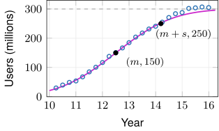
The halfway output is $v + \frac{A}{2} = 0 + \frac{300}{2} = 150$ . The data pass 150 between 138 at Year 12.25 and 151 at Year 12.5, much closer to 12.5. The five-sixths level is $v + \frac{5A}{6} = 0 + \frac{5(300)}{6} = 250$ . The data pass 250 near Year 14.2, between 241 at 14.00 and 255 at 14.25. The two crossings give the mean and the spread:

m = 12.5, \qquad s = x_1 - m = 14.2 - 12.5 = 1.7.

The approximate model is

\text{Users} = 300\cdot\text{\rcmd{pnorm}}(\text{Year}, 12.5, 1.7) + 0.

(b) Plot the data and the approximate model together:

plotPoints(Users ~ Year,
data = TwitterUsers3)
plotFun(300*pnorm(Year, 12.5, 1.7) + 0
~ Year, add = TRUE,
col = "magenta2")

The curve passes within 7 million users of every point through Year 14.5. The curve sits 9 to 18 million below the last five quarters, which shows that the level $R = 300$ is a little low. In the figure, the dashed line is the level on the right, $v + A = 300$ , and the black points are the landmarks $(m, 150) = (12.5, 150)$ and $(m + s, 250) = (14.2, 250)$ .

Example 8

The dataset NetherlandsPopulation, in the MMAC package, records the population of the Netherlands in millions of people at the start of each decade from 1700 to 2010. Approximate the parameters of a sigmoid model for NetherlandsPopulation by hand.

ShowHide solution

Plot the data:

plotPoints(Population ~ Year, data = NetherlandsPopulation)

The data run flat near 1.9 from 1700 to 1800, which rounds to $L = 2$ . The record has no level on the right, because it is still climbing at 16.611 in 2010. The climb slows after 1970: the gain per decade falls from 1.540 million in the 1960s to 0.747 million in the 2000s. The slowing suggests a level above the last value that the record does not show. The value $R = 17$ , a little above the last value 16.611, is a conjecture. The two levels give the vertical shift and the amplitude:

v = 2, \qquad A = 17 - 2 = 15.

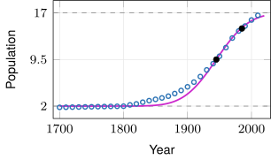
The halfway output is $2 + \frac{15}{2} = 9.5$ . The data pass 9.5 near 1945, between 8.834 in 1940 and 10.027 in 1950. The five-sixths level is $2 + \frac{5(15)}{6} = 14.5$ . The data pass 14.5 near 1985, between 14.091 in 1980 and 14.892 in 1990. The two crossings give the mean and the spread:

m = 1945, \qquad s = 1985 - 1945 = 40.

The approximate model is

\text{Population} = 15\cdot\text{\rcmd{pnorm}}(\text{Year}, 1945, 40) + 2.

In the figure, the dashed lines are the level on the left, $v = 2$ , and the conjectured level on the right, $v + A = 17$ . The black points are the landmarks $(m, 9.5) = (1945, 9.5)$ and $(m + s, 14.5) = (1985, 14.5)$ , and the magenta curve is the approximate model. The data end below the dashed line at 17, the level the record does not show.

Next: 5. Best-Fit Sigmoid Model in R Lesson map

5. Best-Fit Sigmoid Model in R

Objective. In R, use fitModel() to obtain the best-fit sigmoid model.

The function fitModel() searches for the best-fit values of all four parameters, starting from the guesses given in start = list(). After the fit, coef() prints the fitted $A$ , $m$ , $s$ , and $v$ .

R template for a sigmoid fit.

model = fitModel(OUTPUT ~ A*pnorm(INPUT, m, s) + v,
data = DATASET,
start = list(A = AEST, m = MEST, s = SEST, v = VEST))
coef(model)
plotPoints(OUTPUT ~ INPUT, data = DATASET)
plotFun(model(INPUT) ~ INPUT, add = TRUE, col = "red")

Replace DATASET with the dataset’s name, OUTPUT and INPUT with its variable names, and AEST, MEST, SEST, and VEST with the by-hand estimates.

Example 9

Find the best-fit sigmoid model for TwitterUsers3, starting from the estimate

\text{Users} = 300\cdot\text{\rcmd{pnorm}}(\text{Year}, 12.5, 1.7) + 0,

and plot it on the data.

ShowHide solution

Fit the sigmoid model with the estimate’s parameters as starting values:

twitterModel = fitModel(Users ~ A*pnorm(Year, m, s) + v,
data = TwitterUsers3,
start = list(A = 300, m = 12.5, s = 1.7, v = 0))
coef(twitterModel)

The last line prints

A	m	s	v
325.967087	12.624146	1.870371	-3.973658

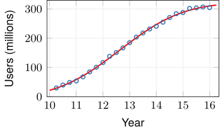
R prints each parameter’s name from the formula above its value. Rounding each value to three decimals and substituting it for its own letter in $y = A\cdot\text{\rcmd{pnorm}}(x, m, s) + v$ gives the best-fit model

\text{Users} = 325.967\cdot\text{\rcmd{pnorm}}(\text{Year}, 12.624, 1.870) - 3.974.

Plot the fitted model function on the data:

plotPoints(Users ~ Year,
data = TwitterUsers3)
plotFun(twitterModel(Year)
~ Year, add = TRUE,
col = "red")

Messages from fitModel().

Object not found. A variable name in the formula is not one of the dataset’s own. Names in R are case sensitive.

> fitModel(users ~ A*pnorm(Year, m, s) + v, data = TwitterUsers3,
+   start = list(A = 300, m = 12.5, s = 1.7, v = 0))
Error in eval(lhs(formula), data) : object 'users' not found

Singular gradient matrix. The function fitModel() stops with this error when the start list is missing, or when a name in it differs from the parameter names in the formula.

> fitModel(Users ~ A*pnorm(Year, m, s) + v, data = TwitterUsers3)
Error in nlsModel(formula, mf, start, wts, scaleOffset = scOff,

nDcentral = nDcntr) :

singular gradient matrix at initial parameter estimates

NaNs produced. The starting guess, here $s = 6$ , is too far off. The search reaches a negative $s$ , where pnorm gives NaN.

> fitModel(Users ~ A*pnorm(Year, m, s) + v, data = TwitterUsers3,
+   start = list(A = 300, m = 12.5, s = 6, v = 0))
Error in numericDeriv(form[[3L]], names(ind), env, central = nDcentral) :

Missing value or an infinity produced when evaluating the model
In addition: Warning message:
In pnorm(Year, m, s) : NaNs produced

Bad fit with no message. The function fitModel() can return a fit that misses the data and print no message. To catch such a fit, plot the fitted curve on the data after every fit, as in Example 9.

Example 10

Find the best-fit sigmoid model for NetherlandsPopulation, starting from the estimate

\text{Population} = 15\cdot\text{\rcmd{pnorm}}(\text{Year}, 1945, 40) + 2.

ShowHide solution

Fit as in Example 9, with the estimate’s parameters as starting values:

dutchModel = fitModel(Population ~ A*pnorm(Year, m, s) + v,
data = NetherlandsPopulation,
start = list(A = 15, m = 1945, s = 40, v = 2))
coef(dutchModel)

The last line prints

A	m	s	v
19.910591	1964.484949	66.819109	1.929576

The best-fit model is

\text{Population} = 19.911\cdot\text{\rcmd{pnorm}}(\text{Year}, 1964.485, 66.819) + 1.930.

The model’s level on the right is $v + A = 1.929576 + 19.910591 \approx 21.840$ million, well above the by-hand level $R = 17$ . The record stops before the population levels off, and the fit sets the level on the right from the shape of the climb alone.

Next: 6. Evaluation and Interpretation Lesson map

6. Evaluation and Interpretation

Objective. Evaluate a sigmoid model at a given input and interpret the answer.

Dataset help entries. The help entry for a dataset, such as ?TwitterUsers3, gives each variable’s units. Those units belong in the interpretation.

Evaluation through the model function. A call such as twitterModel(15) uses the fitted parameters at full precision. Retyping the parameters rounded to three decimals, 325.967*pnorm(15, 12.624, 1.870) - 3.974, shifts the result in the second decimal place.

Recorded rows. To see the recorded rows, type View(TwitterUsers3) in the Console, which opens a table that lists each row with its input value. To pick out a row in R code, compare the input with ==, as in the last line of Example 11.

Units of $m$ and $v + A$ . The mean $m$ is in the input’s units. The level on the right, $v + A$ , is in the output’s units.

Negative fitted $v$ . The fitted $v$ for TwitterUsers3 is about $-3.974$ million users, an impossible number of people. The fit stands as it is, because $v$ is the level the curve approaches far to the left of the recorded inputs. Over the recorded inputs, 10.25 to 16, the model’s outputs run from about 29.327 to 310.407 million users.

Example 11

Use the best-fit sigmoid model for TwitterUsers3 to predict the number of Twitter users at the start of 2015, and compare the prediction with the recorded value.

ShowHide solution

The start of 2015 is Year 15. Fit the model from the by-hand estimates of Example 7, evaluate it at 15, and print the recorded row:

twitterModel = fitModel(Users ~ A*pnorm(Year, m, s) + v,
data = TwitterUsers3,
start = list(A = 300, m = 12.5, s = 1.7, v = 0))
twitterModel(15)
TwitterUsers3[TwitterUsers3$Year == 15, ]

The call twitterModel(15) prints [1] 288.746. The model predicts 288.746 million monthly active Twitter users at the start of 2015. The prediction is an interpolation (Lesson 4 sheet, section 3), because the input 15 lies inside the recorded inputs, 10.25 to 16.

The last line prints row 20 of the data: 288 million users at Year 15. The model misses the recorded value by 0.746 million users.

Example 12

Use the best-fit sigmoid model for NetherlandsPopulation to predict the population of the Netherlands in 2020.

ShowHide solution

Fit the model from the by-hand estimates of Example 8 and evaluate it at 2020:

dutchModel = fitModel(Population ~ A*pnorm(Year, m, s) + v,
data = NetherlandsPopulation,
start = list(A = 15, m = 1945, s = 40, v = 2))
dutchModel(2020)

The last line prints [1] 17.7976. The model predicts a population of 17.798 million people in the Netherlands in 2020. The prediction is an extrapolation, because the year 2020 lies past the last recorded year, 2010.

Example 13

Interpret the mean $m$ and the level on the right $v + A$ of the best-fit sigmoid model for TwitterUsers3,

\text{Users} = 325.967\cdot\text{\rcmd{pnorm}}(\text{Year}, 12.624, 1.870) - 3.974.

ShowHide solution

Fit the model from the by-hand estimates of Example 7 and add the fitted $A$ and $v$ at full precision:

twitterModel = fitModel(Users ~ A*pnorm(Year, m, s) + v,
data = TwitterUsers3,
start = list(A = 300, m = 12.5, s = 1.7, v = 0))
cf = coef(twitterModel)
cf["A"] + cf["v"]

The last line prints 321.9934 under the label A, the first name in the sum. The mean is $m \approx 12.624$ , which places the fastest growth in Twitter users at Year 12.624. Since $0.624 \times 12 \approx 7.5$ months, Year 12.624 is about mid-August 2012. The level on the right is $v + A \approx 321.993$ . The model predicts that monthly active Twitter users level off at 321.993 million.

Lesson map