Rates of Change
Looking ahead
Objectives
- Compute the average rate of change of a function over an interval (slope of a secant line), including dimension and units.
- Compute the average rate of change over multiple small intervals to estimate the instantaneous rate of change at a given input.
- Describe the derivative at a given input as the instantaneous rate of change and as the slope of a tangent line.
- Given a function and a scenario, interpret the meaning of the derivative at a given input, including units.
- Write and understand Lagrange (“prime”) and Leibniz (“fraction”) derivative notation.
- Given a function and input value, give the equation of the tangent line at that input.
1. Average Rate of Change
Objective. Compute the average rate of change of a function over an interval (slope of a secant line), including dimension and units.
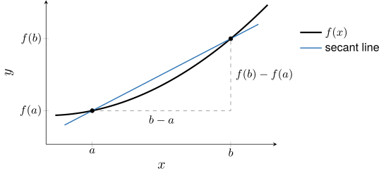
Definition 1 (Average rate of change).
The average rate of change of a function over the interval is the total change in output values of divided by the total change in input values:
A single input has no average rate of change. Over the change in inputs is , and the quotient is undefined; the definition applies only to an interval with .
Definition 2 (Secant line).
A secant line is a line connecting two points on the graph of a function.
The line meets the graph of only at . It is not a secant line, because the definition requires two points on the graph.
The average rate of change of over is the slope of the secant line through and .
Units and dimension. The units of an average rate of change are output units per input unit, as in miles per hour. The dimension is .
When the output is itself a rate, the units of its rate of change have a second “per input unit.” A velocity in meters per second, with time in seconds, has a rate of change in meters per second per second, written m/s. Its dimension follows from the dimension arithmetic of the Lesson 12 Notes, section 3:
Example 1
Compute the average rate of change of over and over :
ShowHide solution
By the definition of average rate of change, the average rate of change of over is
Over , evaluate at the endpoints and :
Substitute and into the formula for the average rate of change:
Over , evaluate at the endpoints and . The output comes from the first interval:
Substitute and into the formula for the average rate of change:
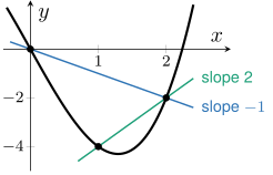
The average rate of change is over and over . The signs differ because lies below and above . By the definition of a secant line, the line through the graph points and is a secant line; it falls with slope , and the secant line through and rises with slope 2.
Example 2
The table gives the median home price in thousands of dollars from 2001 to 2010 (MMAC 4.1 Question 1). Compute the average rate of change in median home price from 2004 to 2007, with its units and dimension.
| Year | 2001 | 2002 | 2003 | 2004 | 2005 | 2006 | 2007 | 2008 | 2009 | 2010 |
| Price | 175.2 | 187.6 | 195.0 | 221.0 | 240.9 | 246.5 | 247.9 | 232.1 | 216.7 | 221.8 |
ShowHide solution
Read the 2004 and 2007 prices from the table and substitute them into the formula for the average rate of change:
The units are thousand dollars per year, and the dimension is . From 2004 to 2007, the median home price rose by an average of about 8.967 thousand dollars, or about $8,967, per year.
Example 3
Compute the average rate of change of over and over in R:
ShowHide solution
Define with makeFun(), then define f_change(a, b), which computes the average rate of change of over from its formula. Evaluate it on each interval. Used R.
f = makeFun(x^3 - 5*x ~ x)
f_change = makeFun((f(b) - f(a))/(b - a) ~ a & b)
f_change(0, 2)
[1] -1
f_change(1, 2)
[1] 2
R returns
Both values match Example 1.
Parentheses. The line f(2) - f(0)/(2 - 0) returns , because R divides by 2 before subtracting. Put the numerator and the denominator each in their own parentheses: (f(2) - f(0))/(2 - 0).
2. Estimating the Instantaneous Rate of Change
Objective. Compute the average rate of change over multiple small intervals to estimate the instantaneous rate of change at a given input.
A car’s average speed over a trip is an average rate of change. The speedometer reading at one moment is an instantaneous rate of change.
Definition 3 (Instantaneous rate of change).
The instantaneous rate of change of a function when is the value approached by the average rates of change of when these rates are computed over smaller and smaller intervals containing . If the average rates of change do not approach a unique, fixed value, then the instantaneous rate of change is undefined when .
The function has no instantaneous rate of change when . For every , its average rate of change over is , and over it is . The average rates from the two sides stay apart, and the definition requires them to approach one unique, fixed value.
Intervals. An interval containing may be symmetric, as in . It may also be one-sided, as in or . When the instantaneous rate of change exists, the average rates over symmetric and one-sided intervals approach the same value.
Stopping test. To estimate the instantaneous rate of change when , follow these steps:
- Compute average rates of change over intervals containing , shrinking , the distance from to the far end of each interval, by a factor of 10 at each step. Early steps may use symmetric intervals; every step tested for stopping uses both one-sided intervals, and .
- Stop at a step where, to three decimals, the two one-sided rates agree with each other and with the rate or rates on the step before. A rounded counts as .
Example 4
Use R to estimate the instantaneous rate of change of when :
ShowHide solution
By the definition of instantaneous rate of change, the rate is the value that the average rates of change approach over smaller and smaller intervals containing . Define and the average-rate function f_change(a, b). Compute average rates of change over symmetric intervals that shrink toward , then over one-sided intervals on each side of , and apply the stopping test. Used R.
f = makeFun(x^3 - 5*x ~ x)
f_change = makeFun((f(b) - f(a))/(b - a) ~ a & b)
f_change(-1, 1)
[1] -4
f_change(-0.1, 0.1)
[1] -4.99
f_change(-0.01, 0.01)
[1] -4.9999
f_change(0, 0.001)
[1] -4.999999
f_change(-0.001, 0)
[1] -4.999999
Rounded to three decimals, the rates over and are and . On the next step both one-sided rates round to : the rounded rate is unchanged, and the rates from the two sides agree. Both conditions of the stopping test are met:
The instantaneous rate of change of when is approximately . The size is reasonable: near the term is tiny, and behaves like the line .
Data tables. At the first or last input of a table, use the one-sided interval between that input and its neighboring input. At an interior input, use the interval between the neighboring inputs on each side. For 2005 in the table of Example 2, that interval is , and the estimate is
thousand dollars per year.
Example 5
The last two entries of a table of median home price in thousands of dollars are 216.7 for 2009 and 221.8 for 2010. Estimate the instantaneous rate of change in median home price in 2010.
ShowHide solution
The year 2010 is the last input in the table. Use the one-sided interval , from the neighboring year to 2010, and substitute its prices into the formula for the average rate of change:
In 2010, the median home price is increasing at about 5.1 thousand dollars, or about $5,100, per year.
3. Derivative
Objective. Describe the derivative at a given input as the instantaneous rate of change and as the slope of a tangent line.
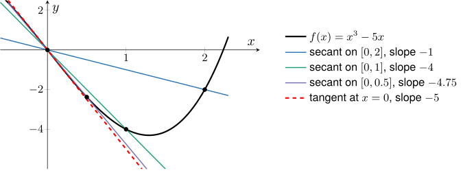
The figure shows secant lines of over , , and . The slope over is , from Example 1. The other two slopes are
As the interval shrinks toward , the slopes approach , the instantaneous rate of change estimated in Example 4, and the secant lines approach the dashed line through with slope . That line is the tangent line, defined next.
Definition 4 (Tangent line).
The tangent line to the graph of a function at the point is the line through whose slope is the instantaneous rate of change of when .
The vertical line meets the graph of only at , and it is not the tangent line there, because a vertical line has no slope. The definition requires a slope equal to the instantaneous rate of change, here about .
Definition 5 (Derivative).
The instantaneous rate of change of a function when is called the derivative of when and is denoted by . The following names are used interchangeably:
- the instantaneous rate of change of when
- the derivative of when
- the rate of change of when
- the slope of the tangent line to when
- the slope of the graph of when
The function has no derivative when , because its instantaneous rate of change there is undefined: its average rates are 1 from the right and from the left, as shown after the definition of instantaneous rate of change.
Height and slope. The output is the height of the graph of at . The derivative is the slope of the tangent line there.
Example 6
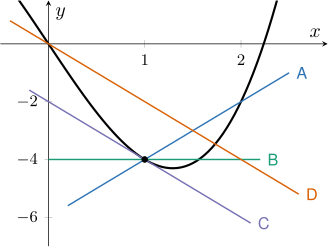
The graph shows four lines near the point on the graph of
The derivative at that point is . Which line is the tangent line to when ?
ShowHide solution
By the definition of a tangent line, the tangent line to when passes through with slope . Line C does both, and it is the tangent line. Line A is not the tangent line. It passes through the graph points and , and its slope is instead of ; it is the secant line over . Line B is not the tangent line, because it is horizontal, with slope 0 instead of . Line D is not the tangent line: it passes through and , with slope , and misses the point .
Example 7
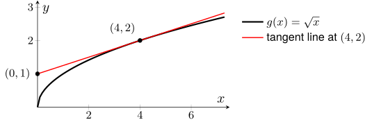
The graph shows and its tangent line at . The tangent line also passes through . Find , and describe it as a slope and as a rate of change.
ShowHide solution
By the definition of a tangent line, the slope of the tangent line at is the instantaneous rate of change of when , which the definition of the derivative names . Compute the slope from the two marked points on the tangent line:
The derivative is the slope of the tangent line at . It is also the instantaneous rate of change: when , is increasing at 0.25 output units per input unit. As a check, the average rate of change over is , close to 0.25.
4. Interpreting the Derivative
Objective. Given a function and a scenario, interpret the meaning of the derivative at a given input, including units.
The height in meters of a ball thrown straight up, seconds after release, is
The graphs show with its tangent line at , 1, 2, and 3. The derivatives are estimated from one-sided average rates on each side of each input. Used R.
H = makeFun(19.6*t - 4.9*t^2 ~ t)
H_change = makeFun((H(b) - H(a))/(b - a) ~ a & b)
H_change(0.5, 0.5001)
[1] 14.69951
H_change(0.4999, 0.5)
[1] 14.70049
H_change(0.5, 0.50001)
[1] 14.69995
H_change(0.49999, 0.5)
[1] 14.70005
H_change(1, 1.0001)
[1] 9.79951
H_change(0.9999, 1)
[1] 9.80049
H_change(1, 1.00001)
[1] 9.799951
H_change(0.99999, 1)
[1] 9.800049
H_change(2, 2.0001)
[1] -0.00049
H_change(1.9999, 2)
[1] 0.00049
H_change(2, 2.00001)
[1] -4.899974e-05
H_change(1.99999, 2)
[1] 4.900009e-05
H_change(3, 3.0001)
[1] -9.80049
H_change(2.9999, 3)
[1] -9.79951
H_change(3, 3.00001)
[1] -9.800049
H_change(2.99999, 3)
[1] -9.799951
At each input, the two one-sided rates over intervals of width 0.0001 and of width 0.00001 all round to the same value to three decimals, with counted as . The stopping test is met: , , , and . The graphs round these to one decimal.
Positive derivative
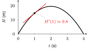
The derivative is positive, and the tangent line rises. One second after release, the ball’s height is increasing at about 9.8 meters per second.
Negative derivative
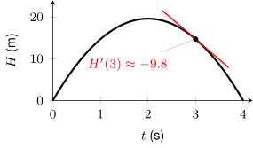
The derivative is negative, and the tangent line falls. Three seconds after release, the ball’s height is decreasing at about 9.8 meters per second.
Zero derivative
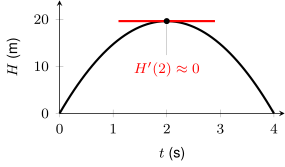
The derivative is approximately 0, and the tangent line is horizontal. Two seconds after release, the ball’s height is neither increasing nor decreasing: the ball is at the top of its flight.
Size of the derivative
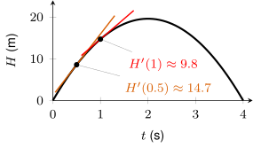
The derivative is larger than , and the orange tangent line at is steeper than the red one at . Half a second after release, the ball’s height is increasing at about 14.7 meters per second, a rate of greater size than the 9.8 meters per second at one second.
Interpretation. An interpretation of is one sentence that states
- the input value, with its units,
- whether the output is increasing or decreasing, and
- the size of the rate of change, , in output units per input unit.
For a zero derivative at a peak or a valley of the graph, the output is neither increasing nor decreasing. A zero derivative can also occur where the output keeps increasing: has and is increasing through .
Example 8
The function Weight models the average weight in grams of a male fetus, with input Week the gestational age in weeks:
Estimate in R from average rates of change on both sides of week 26, starting with and . Give its units and dimension, and interpret it (MMAC 4.1 Exercise 76).
ShowHide solution
Estimate the derivative as in Example 4, with one-sided intervals on each side of week 26 that shrink by a factor of 10. Used R.
Weight = makeFun(781.9*exp(0.1216*(Week - 25)) ~ Week)
Weight_change = makeFun((Weight(b) - Weight(a))/(b - a) ~ a & b)
Weight_change(26, 26.0001)
[1] 107.3736
Weight_change(25.9999, 26)
[1] 107.3723
Weight_change(26, 26.00001)
[1] 107.373
Weight_change(25.99999, 26)
[1] 107.3729
Weight_change(26, 26.000001)
[1] 107.373
Weight_change(25.999999, 26)
[1] 107.373
The rates round to 107.374 and 107.372 on the first step and to 107.373 on both sides on the next two. The stopping test is met:
The units are grams per week, and the dimension is
In week 26, the average male fetus’s weight is increasing at about 107.373 grams per week. As a check, the average rate over is grams per week, close to the estimate.
Example 9
The temperature Temp in degrees Fahrenheit on a spring day is modeled by
with input Hour the hour of the day on a 24-hour clock. Use R to estimate , , and , and interpret each.
ShowHide solution
Estimate each derivative as in Example 4, with one-sided intervals on each side of the hour. Used R.
Temp = makeFun(60 - 0.5*(Hour - 14)^2 ~ Hour)
Temp_change = makeFun((Temp(b) - Temp(a))/(b - a) ~ a & b)
Temp_change(10, 10.0001)
[1] 3.99995
Temp_change(9.9999, 10)
[1] 4.00005
Temp_change(10, 10.00001)
[1] 3.999995
Temp_change(9.99999, 10)
[1] 4.000005
Temp_change(12, 12.0001)
[1] 1.99995
Temp_change(11.9999, 12)
[1] 2.00005
Temp_change(12, 12.00001)
[1] 1.999995
Temp_change(11.99999, 12)
[1] 2.000005
Temp_change(14, 14.0001)
[1] -4.999997e-05
Temp_change(13.9999, 14)
[1] 4.999997e-05
Temp_change(14, 14.00001)
[1] -5.000089e-06
Temp_change(13.99999, 14)
[1] 5.000089e-06
R prints the rates at hour 14 in scientific notation: -4.999997e-05 is . The rates at each hour round to the same value on both sides and on both steps. At hour 14 the right-side rates round to , which counts as , and the stopping test is met:
At 1000, the temperature is increasing at about 4.000 degrees Fahrenheit per hour. At 1200, it is increasing at about 2.000 degrees Fahrenheit per hour, half the rate at 1000. At 1400, the temperature is neither increasing nor decreasing: it is at the day’s high, degrees Fahrenheit.
5. Derivative Notation
Objective. Write and understand Lagrange (“prime”) and Leibniz (“fraction”) derivative notation.
| Notation | Symbol | Pronunciation |
|---|---|---|
| Lagrange (“prime”) | “ prime of ” | |
| Leibniz (“fraction”) | “ evaluated at ” |
The Leibniz fraction is written like an average rate of change, the change in outputs divided by the change in inputs. The derivative is the value that these average rates approach as the intervals shrink. The bar with at its lower right marks the input where the derivative is taken. The fraction gives the dimension of the derivative as .
Inverse notation. The symbols and name different objects. The superscript in marks the inverse function evaluated at , and the prime in marks the derivative of when .
Example 10
The function Weight models the average weight in grams of a male fetus, with input Week the gestational age in weeks, and satisfies . Write this derivative in Leibniz notation and give its dimension from the fraction.
ShowHide solution
In Leibniz notation, the derivative is
The dimension is
Example 11
The height in meters of a ball thrown straight up, seconds after release, satisfies
Write this derivative in Lagrange notation, say it aloud, and give its units and dimension.
ShowHide solution
In Lagrange notation, the derivative is , read “ prime of 3.” The units are meters per second, and the Leibniz fraction gives the dimension:
6. Equation of the Tangent Line
Objective. Given a function and input value, give the equation of the tangent line at that input.
Definition 6 (Equation of the tangent line).
The equation of the tangent line to at is given by
- Calculate .
- Calculate or approximate .
- Substitute these values into the equation of the tangent line.
A line through the point with slope has the equation , its point-slope form. The equation of the tangent line is that form with , solved for . Distributing and collecting the constants gives the slope-intercept form: the slope times plus the vertical intercept, as in .
A horizontal line passes through , and it is not the tangent line when , because its slope 0 differs from .
Example 12
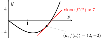
Find the equation of the tangent line to when , with estimated in R:
ShowHide solution
The equation of the tangent line to at is
here with . To write the equation, find the output , the height of the point of tangency, and the slope . Calculate the output by hand:
Estimate as in Example 4, with one-sided intervals on each side of . Used R.
f = makeFun(x^3 - 5*x ~ x)
f_change = makeFun((f(b) - f(a))/(b - a) ~ a & b)
f_change(2, 2.001)
[1] 7.006001
f_change(1.999, 2)
[1] 6.994001
f_change(2, 2.0001)
[1] 7.0006
f_change(1.9999, 2)
[1] 6.9994
f_change(2, 2.00001)
[1] 7.00006
f_change(1.99999, 2)
[1] 6.99994
f_change(2, 2.000001)
[1] 7.000006
f_change(1.999999, 2)
[1] 6.999994
The rates round to 7.006 and 6.994 on the first step, to 7.001 and 6.999 on the second, and to 7.000 on both sides on the last two. The stopping test is met:
Substitute and into the equation of the tangent line, then distribute and collect the constants:
As a check, the line passes through the point of tangency: . On the graph, the tangent line touches at and climbs with slope .
Example 13
The function Weight models the average weight in grams of a male fetus, with input Week the gestational age in weeks:
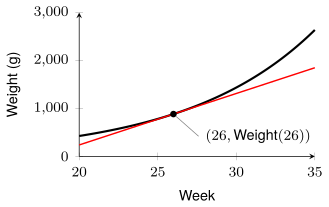
Find the equation of the tangent line at week 26 in slope-intercept form, and plot it with the model in R.
ShowHide solution
The slope is , from Example 8. Distribute in the equation of the tangent line to reach slope-intercept form:
Compute the vertical intercept in R twice, with first from the right-side rate and then from the left-side rate, to confirm that the two sides give the same intercept. Keep at full precision, because multiplying by 26 multiplies its rounding error by 26. Used R.
Weight = makeFun(781.9*exp(0.1216*(Week - 25)) ~ Week)
Weight_change = makeFun((Weight(b) - Weight(a))/(b - a) ~ a & b)
m = Weight_change(26, 26.000001)
Weight(26) - 26*m
[1] -1908.696
m = Weight_change(25.999999, 26)
Weight(26) - 26*m
[1] -1908.696
Both sides give . By hand, with and rounded to three decimals, the computation is
The hand result differs from R’s in the last decimal, the rounding error that R avoids by keeping and at full precision. The tangent line is
Plot the model and the tangent line together. Used R.
tangent = makeFun(Weight(26) + m*(Week - 26) ~ Week)
plotFun(Weight(Week) ~ Week, xlim = range(20, 35))
plotFun(tangent(Week) ~ Week, add = TRUE, col = "red")
R’s plot shows the model curve and, with col = "red", the tangent line in red, as in the figure. The red line is , and it touches the model at . At week 27 the tangent line’s value is grams, below the model’s grams, because the model curves upward.
Found a mistake, a broken tool or something unclear? Report a problem