Chain Rule II

• For $(3\cos(x) - e^x)^5$: the chain rule with the basic rules, because the function is a composition, a power of the difference $3\cos(x) - e^x$.
• For $(2\sin(x) + 5)(x^3 - 4)$: the product or quotient rule with the basic rules, because the function is a product of two factors, and each factor is differentiated by the basic rules.
• For $\ln(x) - \sin(x) + 4e^x$: the basic rules only, because every term is a basic modeling function of $x$ or a constant times a basic modeling function.
• For $e^{x^2\cos(3x)}$: the product or quotient rule and the chain rule with the basic rules, because the outside function $e^x$ takes the product $x^2\cos(3x)$ as input, and the factor $\cos(3x)$ is a composition.
• For $-3\sqrt{1 + x^2}$: the chain rule with the basic rules, because the function is the constant $-3$ times the composition $\sqrt{1 + x^2}$.
• For $\cos(\ln(x^2 + 4))$: the chain rule with the basic rules, because the function is a composition of three functions: the outside function $\cos(x)$, the middle function $\ln(x)$, and the inside function $x^2 + 4$.

The inside function is $g(x) = 3\cos(x) - e^x$, with $g'(x) = -3\sin(x) - e^x$. The outside function is $f(x) = x^5$, with $f'(x) = 5x^4$. The chain rule, $p'(x) = f'(g(x))\cdot g'(x)$, then gives

The derivatives of the two factors are

The product rule (Lesson 30 section 2) is

With the first factor $2\sin(x) + 5$ in place of $f(x)$ and the second factor $x^3 - 4$ in place of $g(x)$,

The function is the product of $7\sin(4x)$ and $e^{-2x}$. Differentiate each factor, then apply the product rule. The first factor is differentiated by the chain rule, with inside function $4x$ and outside function $7\sin(x)$. The second factor is differentiated by the extended exponential rule:

Substitute both factors and their derivatives into the product rule, and factor out $14e^{-2x}$:

The function is a quotient. Differentiate the numerator and the denominator, then apply the quotient rule. The numerator is differentiated by the chain rule, with inside function $x^2$ and outside function $\cos(x)$. The denominator is differentiated by the extended exponential rule:

The quotient rule (Lesson 30 section 2) is

Substitute the numerator $\cos(x^2)$ for $f(x)$ and the denominator $e^{2x}$ for $g(x)$, then cancel the factor $e^{2x}$ common to every term:

Rewrite the cube root as a power:

The inside function is $g(x) = x^2 - 4x + 9$, with $g'(x) = 2x - 4$. The outside function is $f(x) = -6x^{1/3}$, with

The constant $-6$ stays in the outside function, as in section 2 of the Lesson 32 Notes. Substitute into the chain rule, distribute $-2$, and move the negative power to the denominator:

The inside function is $h(x) = 3\ln(x) + 2$, with $h'(x) = \frac{3}{x}$. The middle function is $g(x) = x^4$, with $g'(x) = 4x^3$. The outside function is $f(x) = \cos(x)$, with $f'(x) = -\sin(x)$. In the diagram, the arrows run from $x$ through $h$, $g$, and $f$ in turn. Under each function is its factor in the derivative.

By the chain rule for three functions, $k'(x)$ is the product of the three factors:

which gives

The inside function is the product $g(x) = x^2\cos(3x)$. Find $g'$ by the product rule, then substitute $g'$ into the chain rule for $e^{g(x)}$. The factor $x^2$ has derivative $2x$. The factor $\cos(3x)$ is itself a composition, with derivative $-\sin(3x)\cdot 3 = -3\sin(3x)$ by the chain rule. By the product rule,

The outside function is $f(x) = e^x$, with $f'(x) = e^x$. Substitute into the chain rule:

Define Temp and differentiate it with D() to get dTemp, R’s name for $\text{Temp}'$. Evaluate both at month 28, and evaluate Temp at months 27 and 29. Used R.

Temp = makeFun(23.3*sin(2*pi/11.98*(M - 3.16)) + 65.4 ~ M)
dTemp = D(Temp(M) ~ M)
Temp(28)
[1] 75.77605
dTemp(28)
[1] 10.94161
Temp(27)
[1] 63.93454
Temp(29)
[1] 84.82823

Month 28 is May 2008, since month 24 is January 2008. At the beginning of May 2008, the model gives an average maximum temperature in central Kentucky of about 75.776 degrees Fahrenheit: $\text{Temp}(28) \approx 75.776$.

At month 28, the model’s average maximum temperature is increasing at about 10.942 degrees Fahrenheit per month: $\text{Temp}'(28) \approx 10.942$.

As a check, the rate lies between the model’s changes over the months before and after month 28:

It should, because $\text{Temp}'$ falls toward zero on the approach to the next peak.

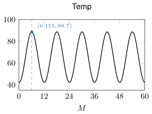
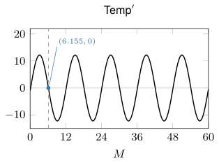
Define Temp and differentiate it with D() to get dTemp, R’s name for $\text{Temp}'$. Plot each on $0 \le M \le 60$. Used R.

Temp = makeFun(23.3*sin(2*pi/11.98*(M - 3.16))

+ 65.4 ~ M)

dTemp = D(Temp(M) ~ M)

plotFun(Temp(M) ~ M, xlim = range(0, 60))

plotFun(dTemp(M) ~ M, xlim = range(0, 60))

The derivative $\text{Temp}'$ is zero at each peak and trough of Temp, because the tangent line to the graph of Temp is horizontal at each peak and trough. Sine reaches its maximum, 1, when its input is $\pi/2$. The first peak of Temp with $M \ge 0$ comes where

$$\frac{2\pi}{11.98}(M - 3.16) = \frac{\pi}{2}.$$

Multiply both sides by $\frac{11.98}{2\pi}$, then add 3.16:

$$M - 3.16 = \frac{11.98}{4}, \qquad M = 3.16 + 2.995 = 6.155.$$

The input $\pi/2 - 2\pi$ gives $M = 6.155 - 11.98 < 0$. The peak value of Temp is $23.3(1) + 65.4 = 88.7$. Each of R’s two plots appears here with a dashed line and a marked point added. The dashed line marks $M = 6.155$ on both graphs: Temp is at its peak, and $\text{Temp}'$ is zero. The derivative $\text{Temp}'$ is positive just to the left of the line, where Temp rises, and negative just to the right, where Temp falls.

Evaluate the hand derivative at each input, using $\sin(1) \approx 0.841471$, $\cos(1) \approx 0.540302$, and $e^2 \approx 7.389056$, with sine and cosine in radians.

Define $q$ and differentiate it with D() to get dq, R’s name for $q'$. Evaluate dq at the same inputs. Used R.

q = makeFun(cos(x^2) / exp(2*x) ~ x)
dq = D(q(x) ~ x)
dq(0)
[1] -2
dq(1)
[1] -0.3740054

At $x = 0$, R gives the hand value $-2$ exactly. At $x = 1$, R’s value rounds to the hand value $-0.374$. The agreement at both inputs supports the hand derivative.