Lesson 28: The Derivative as a Function II

Objectives

Describe differentiable and identify at what inputs a function is or is not differentiable.
Given a function, use R to approximate and plot its first and higher-order derivatives.
Given a first derivative, identify where the function is increasing or decreasing and identify local extrema.
Given a first or second derivative, determine concavity and identify inflection points.

Linked Derivative Graphs Open full screen

1. Differentiability

Objective. Describe differentiable and identify at what inputs a function is or is not differentiable.

Definition 1 (Differentiable).

A function $f(x)$ is differentiable at $x = a$ if and only if the derivative $f'(a)$ exists. A function $f(x)$ is differentiable on an interval if and only if $f(x)$ is differentiable at every input in the interval.

The function $f(x) = |x|$ is not differentiable at $x = 0$ , because the derivative $f'(0)$ does not exist. Its average rates of change approach 1 from the right and $-1$ from the left (Lesson 26 Notes, Example 11).

Graphical features that correspond to a function being nondifferentiable are sharp points, including corners and cusps, as well as breaks in the graph, including holes, jumps, and vertical asymptotes. Each graph below is the graph $y = f(x)$ of a function $f$ with one feature at $x = 0$ .

Corner

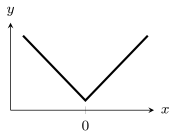
The slopes on the two sides of $x = 0$ are different numbers, $-1$ and 1.

Cusp

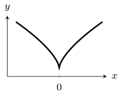
The graph comes to a sharp point, and near $x = 0$ the slopes grow without bound in size.

Hole

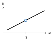
The derivative $f'(0)$ does not exist, because $f(0)$ is undefined and the limit definition of the derivative uses $f(0)$ .

Jump

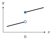
The filled dot is $f(0)$ , and the outputs from the left approach a lower value. Over a short interval $[x, 0]$ on the left, the change in output stays near the height of the jump while the interval’s length shrinks toward 0. Their quotient, the average rate of change, grows without bound.

Vertical asymptote

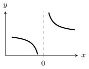
The function has no output at $x = 0$ , and near $x = 0$ its outputs grow without bound in size.

Example 1

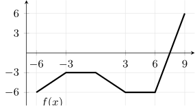
Sketch the graph of the derivative of the function $f(x)$ graphed below, and identify the inputs $x$ with $-6 < x < 9$ where $f$ is not differentiable.

ShowHide solution

By the definition of differentiable, $f$ is differentiable at $x = a$ exactly when $f'(a)$ exists. On each of the five line segments, $f'(x)$ is the slope of the segment:

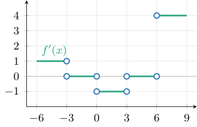
f'(x) = \begin{cases} 1 & -6 < x < -3 \\ 0 & -3 < x < 0 \\ -1 & 0 < x < 3 \\ 0 & 3 < x < 6 \\ 4 & 6 < x < 9 \end{cases}.

Each slope is the rise over the run, such as $\frac{6 - (-6)}{9 - 6} = 4$ on the last segment. At $x = -3$ , every interval $[x, -3]$ with $-6 \le x < -3$ gives an average rate of change of $1$ , and every interval $[-3, x]$ with $-3 < x \le 0$ gives $0$ . Because the left and right average rates of change approach different numbers, $f'(-3)$ does not exist. The slopes on the two sides of $x = 0$ , $x = 3$ , and $x = 6$ also differ. Therefore, $f$ is not differentiable at $x = -3$ , $0$ , $3$ , and $6$ . The graph beside this text is the sketch of $f'$ : one horizontal segment at the height of each slope, with open dots at the four inputs where $f'$ does not exist.

Example 2

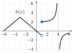
Identify the inputs $x$ with $-6 < x < 6$ where the function $h(x)$ graphed below is not differentiable, and name the graphical feature at each one.

ShowHide solution

The function $h$ is not differentiable at $x = -3$ , $-1$ , $1$ , and $4$ .

The graph of $h$ has a corner at $x = -3$ , because the slope of $h$ is $1$ on the left and $-1$ on the right.
The graph of $h$ has a hole at $x = -1$ , because the outputs approach $1$ from both sides and $h(-1)$ is undefined.
The graph of $h$ has a jump at $x = 1$ , because the outputs approach $-1$ from the left and $2$ from the right.
The graph of $h$ has a vertical asymptote at $x = 4$ , because the outputs grow without bound as $x$ approaches $4$ from the left and fall without bound from the right.

Lesson map

2. Higher-Order Derivatives in R

Objective. Given a function, use R to approximate and plot its first and higher-order derivatives.

Definition 2 (Second and higher-order derivatives).

The second derivative $f''(x)$ of a function $f(x)$ is the derivative of $f'(x)$ . In general, $f^{(1)}(x)$ means $f'(x)$ , and for each integer $n$ with $n \ge 2$ , the $n$ th derivative $f^{(n)}(x)$ of $f(x)$ is the derivative of $f^{(n-1)}(x)$ . The derivatives $f^{(n)}(x)$ with $n \ge 2$ are the higher-order derivatives of $f(x)$ .

The function $f(x) = |x|$ has no second derivative at $x = 0$ , because $f'(0)$ does not exist. The derivative $f'(x)$ is $-1$ for $x < 0$ and 1 for $x > 0$ , and the derivative of $f'$ at $x = 0$ uses the value $f'(0)$ .

Compared with the dimension of $f'(x)$ , the dimension of $f''(x)$ has one more factor of $[\text{input}]^{-1}$ :

[f'(x)] = [\text{output}]\cdot[\text{input}]^{-1}, \qquad [f''(x)] = [\text{output}]\cdot[\text{input}]^{-2}.

The Lesson 25 Notes, section 1, give the units of a rate of a rate, such as an acceleration in m/s $^2$ with dimension $LT^{-2}$ .

Example 3

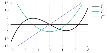
Use R to approximate and plot the first and second derivatives of

f(x) = x^3 - 5x

on $-3 \le x \le 3$ , and estimate $f'(2)$ and $f''(2)$ .

ShowHide solution

By the definition of the second derivative, $f''$ is the derivative of $f'$ . Define $f$ and the step-0.001 approximation f_deriv of $f'$ . The function f_deriv2 applies the same approximation to f_deriv and so approximates $f''$ . Plot all three on $-3 \le x \le 3$ . Used R.

f = makeFun(x^3 - 5*x ~ x)
plotFun(f(x) ~ x, xlim = range(-3, 3), col = "black")
f_deriv = makeFun((f(x + 0.001) - f(x))/0.001 ~ x)
f_deriv2 = makeFun((f_deriv(x + 0.001) - f_deriv(x))/0.001 ~ x)
plotFun(f_deriv(x) ~ x, col = "darkgreen", add = TRUE)
plotFun(f_deriv2(x) ~ x, col = "purple", add = TRUE)

In the plot, the black cubic is $f$ , the green parabola is $f'$ , and the purple line is $f''$ . The parabola crosses the $x$ -axis at the inputs where the cubic has slope 0, and the line crosses the $x$ -axis at $x = 0$ , where the parabola has slope 0.

Evaluate both approximations at $x = 2$ . Used R.

f_deriv(2)
[1] 7.006001
f_deriv2(2)
[1] 12.006

The step-0.001 values 7.006 and 12.006 are first estimates. To find $f'(2)$ and $f''(2)$ to three decimals, apply the stopping test of the Lesson 25 Notes, section 2: shrink the step on both sides of $x = 2$ until the third decimal stops changing.

The second expression below repeats the computation of f_deriv2 with step $h$ . Its part (f(2 + 2*h) - f(2 + h))/h is the first-derivative estimate at $2 + h$ , and (f(2 + h) - f(2))/h is the first-derivative estimate at 2. Their difference divided by $h$ is the average rate of change of the first-derivative estimates from 2 to $2 + h$ , which approximates $f''(2)$ . The three negative entries of h are steps to the left of 2. Used R.

h = c(0.0001, 0.00001, 0.000001, -0.0001, -0.00001, -0.000001)
(f(2 + h) - f(2))/h
[1] 7.000600 7.000060 7.000006 6.999400 6.999940 6.999994
((f(2 + 2*h) - f(2 + h))/h - (f(2 + h) - f(2))/h)/h
[1] 12.00060 12.00004 11.99751 11.99940 11.99997 11.99840

The first-derivative estimates round to $7.000$ from both sides at steps 0.00001 and 0.000001. The stopping test is met:

f'(2) \approx 7.000.

The second-derivative estimates round to $12.000$ from both sides at step 0.00001, and at step 0.000001 they drift to $11.998$ . At so small a step, the rounding error in R’s stored outputs of $f$ is divided by $h$ twice in the formula, and the result is large enough to change the third decimal. The stopping test therefore does not confirm $f''(2)$ . The step-0.00001 estimates come before that drift, and they give the estimate:

f''(2) \approx 12.000.

Example 4

The height $H$ in meters of a ball thrown straight up, $t$ seconds after release, is

H(t) = 19.6t - 4.9t^{2}.

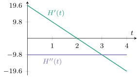
Use R to approximate $H'(1)$ and $H''(1)$ with step 0.001, give the units of each, and plot $H'$ and $H''$ for $0 \le t \le 4$ .

ShowHide solution

Define $H$ and the step-0.001 approximation H_deriv of $H'$ , then H_deriv2, which applies the same approximation to H_deriv. Evaluate both at $t = 1$ , then plot both. Used R.

H = makeFun(19.6*t - 4.9*t^2 ~ t)
H_deriv = makeFun((H(t + 0.001) - H(t))/0.001 ~ t)
H_deriv2 = makeFun((H_deriv(t + 0.001) - H_deriv(t))/0.001 ~ t)
H_deriv(1)
[1] 9.7951
H_deriv2(1)
[1] -9.8
plotFun(H_deriv(t) ~ t, xlim = range(0, 4), col = "darkgreen")
plotFun(H_deriv2(t) ~ t, col = "purple", add = TRUE)

At step 0.001 the error of the estimate of $H'(1)$ shows in the second decimal. Report it to one decimal:

H'(1) \approx 9.8, \qquad H''(1) \approx -9.800.

The derivative $H'$ is the ball’s velocity, in meters per second. The second derivative $H''$ is the rate of change of the velocity, in meters per second per second, written m/s $^2$ , with dimension $LT^{-2}$ . One second after release, the height is increasing at about 9.8 m/s, and the velocity is decreasing at about 9.800 m/s $^2$ .

In the plot, the green line $H'$ falls from about 19.6 to about $-19.6$ . The purple line $H''$ stays at height $-9.8$ at every time.

Third and higher derivatives in R. To approximate each further derivative in R, apply the same step-0.001 formula to the approximation of the derivative before it. The line below defines an approximation of the third derivative $f'''(x)$ , also written $f^{(3)}(x)$ .

f_deriv3 = makeFun((f_deriv2(x + 0.001) - f_deriv2(x))/0.001 ~ x)

Order of the R lines. The function f_deriv2 calls f_deriv, and f_deriv calls f. Evaluating or plotting f_deriv2 before f_deriv is defined gives an error:

> f_deriv2(1)
Error in f_deriv(x + 0.001) : could not find function "f_deriv"

Lesson map

3. Increasing, Decreasing, and Local Extrema

Objective. Given a first derivative, identify where the function is increasing or decreasing and identify local extrema.

Theorem 3 (Derivative and monotonicity).

If $f'(x) > 0$ for every $x$ in an interval, then $f$ is increasing on that interval. If $f'(x) < 0$ for every $x$ in an interval, then $f$ is decreasing on that interval. If $f'(x) = 0$ for every $x$ in an interval, then $f$ is constant on that interval.

Definition 4 (Local extrema).

For a function $f(x)$ and a real number $c$ in its domain, a local maximum is a value $f(c)$ such that $f(c) \geq f(x)$ for all inputs $x$ near input $c$ .

For a function $f(x)$ and a real number $c$ in its domain, a local minimum is a value $f(c)$ such that $f(c) \leq f(x)$ for all inputs $x$ near input $c$ .

A local extremum is a local maximum or a local minimum of $f(x)$ .

The plural is local extrema.

The value $f(0) = 0$ of $f(x) = x^3$ is not a local extremum, because the definition requires $f(0) \ge f(x)$ for every nearby input, or $f(0) \le f(x)$ for every nearby input. Every interval around $x = 0$ contains inputs $x$ with $x > 0$ , where $f(x) = x^3 > 0$ , and inputs $x$ with $x < 0$ , where $f(x) = x^3 < 0$ .

Theorem 5 (Sign test for local extrema).

Let $f$ be continuous at an input $c$ . If $f'$ changes from positive to negative at $c$ , then $f(c)$ is a local maximum. If $f'$ changes from negative to positive at $c$ , then $f(c)$ is a local minimum. If $f'$ has the same sign on both sides of $c$ , then $f$ has no local extremum at $c$ .

A function that is differentiable at an input is continuous there. The sign test therefore applies at every input $c$ where $f'(c)$ exists.

Each graph below shows $f$ near an input $c$ , with the sign of $f'$ on each side.

Local maximum

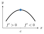
The graph rises to $(c, f(c))$ and then falls, and $f(c)$ is a local maximum.

Local minimum

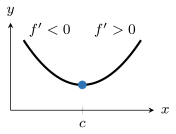
The graph falls to $(c, f(c))$ and then rises, and $f(c)$ is a local minimum.

No local extremum

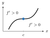
The graph rises on both sides of $c$ , and $f(c)$ is neither a local maximum nor a local minimum.

Breaks in the graph. The sign test for local extrema applies only where $f$ is continuous. The function $h$ in Example 2 falls to the left of its jump at $x = 1$ and rises to the right. The value $h(1) = 2$ is neither a local maximum nor a local minimum, because the outputs just left of $x = 1$ are near $-1$ and the outputs just right of $x = 1$ are above $2$ .

Intervals and local extrema from $f'$ .

Find the inputs where $f'(x) = 0$ or where $f'(x)$ does not exist.
Evaluate $f'$ at one test input inside each interval those inputs mark off.
Label each interval increasing or decreasing by the sign of its test value.
At each input where $f$ is continuous, report a local maximum where $f'$ changes from positive to negative and a local minimum where $f'$ changes from negative to positive.

Example 5

The derivative of $f(x) = x^3 - 5x$ is

f'(x) = 3x^2 - 5.

Identify where $f$ is increasing or decreasing, and identify its local extrema.

ShowHide solution

Because the derivative $f'(x)$ exists at every input, $f$ is continuous everywhere, and the sign test for local extrema applies at every input. Find the inputs where $f'(x) = 0$ by setting $3x^2 - 5 = 0$ :

x^2 = \frac{5}{3} \quad\text{so}\quad x = \pm\sqrt{5/3} \approx \pm 1.291.

Evaluate $f'$ at one test input in each of the three intervals those inputs mark off:

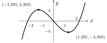
f'(-2) = 3(-2)^2 - 5 = 7, \qquad f'(0) = 3(0)^2 - 5 = -5, \qquad f'(2) = 3(2)^2 - 5 = 7.

Therefore, $f$ is increasing on $(-\infty, -\sqrt{5/3})$ and $(\sqrt{5/3}, \infty)$ and decreasing on $(-\sqrt{5/3}, \sqrt{5/3})$ . Because the sign of $f'$ changes from positive to negative at $x = -\sqrt{5/3}$ , $f$ has a local maximum there. By the definition of local extrema, the local maximum is the value $f\bigl(-\sqrt{5/3}\bigr)$ :

f\bigl(-\sqrt{5/3}\bigr) = \bigl(-\sqrt{5/3}\bigr)^3 - 5\bigl(-\sqrt{5/3}\bigr) = -\tfrac{5}{3}\sqrt{5/3} + 5\sqrt{5/3} = \tfrac{10}{3}\sqrt{5/3} \approx 4.303.

Because the sign of $f'$ changes from negative to positive at $x = \sqrt{5/3}$ , $f$ has a local minimum there, and the local minimum is the value $f\bigl(\sqrt{5/3}\bigr)$ :

f\bigl(\sqrt{5/3}\bigr) = \bigl(\sqrt{5/3}\bigr)^3 - 5\sqrt{5/3} = \tfrac{5}{3}\sqrt{5/3} - 5\sqrt{5/3} = -\tfrac{10}{3}\sqrt{5/3} \approx -4.303.

On the graph of $f$ , the local maximum, about 4.303, is the height of the peak at about $(-1.291, 4.303)$ , and the local minimum, about $-4.303$ , is the height of the valley at about $(1.291, -4.303)$ .

Example 6

The derivative of a function $f(x)$ is

f'(x) = (x + 1)^2(x - 2).

Identify where $f$ is increasing or decreasing, and identify the inputs of its local extrema.

ShowHide solution

The derivative is zero at $x = -1$ and $x = 2$ , where the factors $(x + 1)^2$ and $x - 2$ are zero. Evaluate $f'$ at a test input in each interval, as in Example 5:

f'(-2) = (-1)^2(-4) = -4, \qquad f'(0) = (1)^2(-2) = -2, \qquad f'(3) = (4)^2(1) = 16.

Therefore, $f$ is decreasing on $(-\infty, -1)$ and $(-1, 2)$ and increasing on $(2, \infty)$ . Because the derivative exists at every input, $f$ is continuous everywhere. The function $f$ has a local minimum at $x = 2$ , because $f'$ changes from negative to positive there. The function has no local extremum at $x = -1$ , because $f'$ is negative on both sides.

A rising graph of $f'$ below the $x$ -axis. A graph of $f'$ that rises can be misread as a sign that $f$ is increasing. On $(0, \sqrt{5/3})$ , the graph of $f'(x) = 3x^2 - 5$ from Example 5 rises while its values stay negative. The function $f$ is decreasing on $(0, \sqrt{5/3})$ , because $f'(x) < 0$ for every $x$ in that interval.

Lesson map

4. Concavity and Points of Inflection

Objective. Given a first or second derivative, determine concavity and identify inflection points.

Concave up

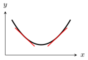
The red segments are tangent lines. Where $f'' > 0$ , their slopes $f'$ increase from left to right, and the graph bends upward.

Concave down

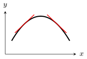
The red segments are tangent lines. Where $f'' < 0$ , their slopes $f'$ decrease from left to right, and the graph bends downward.

Point of inflection

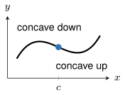
The graph changes from concave down to concave up at $(c, f(c))$ , where $f''$ changes sign.

Definition 6 (Concavity).

For a function $f(x)$ differentiable on the interval $(a,b)$ , $f(x)$ is concave up on $(a,b)$ if and only if $f'(x)$ is increasing on $(a,b)$ .

For a function $f(x)$ differentiable on the interval $(a,b)$ , $f(x)$ is concave down on $(a,b)$ if and only if $f'(x)$ is decreasing on $(a,b)$ .

For a differentiable function, these definitions of concave up and concave down agree with the definitions in the Lesson 5 Notes.

On every interval, the line $f(x) = 2x + 1$ is neither concave up nor concave down, because the definitions require $f'$ to increase or to decrease and its derivative is the constant slope $f'(x) = 2$ .

Definition 7 (Point of inflection).

The point $(c, f(c))$ is a point of inflection of $f(x)$ if and only if $f(x)$ changes concavity at input $c$ .

The point $(0, 0)$ on the graph of $y = x^2$ is not a point of inflection, because the definition requires a change of concavity and the graph is concave up on both sides of $x = 0$ .

Theorem 8 (Second derivative and concavity).

If $f''(x) > 0$ for every $x$ in an interval, then $f$ is concave up on that interval. If $f''(x) < 0$ for every $x$ in an interval, then $f$ is concave down on that interval. If $f''$ changes sign at an input $c$ and $f$ is continuous at $c$ , then $(c, f(c))$ is a point of inflection of $f$ .

The first two sentences of the theorem follow from the derivative and monotonicity theorem with $f'$ in place of $f$ , together with the definition of concavity. Where $f'' > 0$ , the derivative $f'$ is increasing, and by the definition of concavity, $f$ is concave up. Where $f'' < 0$ , the derivative $f'$ is decreasing, and $f$ is concave down.

Concavity and points of inflection from $f''$ .

Find the inputs where $f''(x) = 0$ or where $f''(x)$ does not exist.
Evaluate $f''$ at one test input inside each interval those inputs mark off.
Label each interval concave up or concave down by the sign of its test value.
Report a point of inflection $(c, f(c))$ at each input $c$ where the sign of $f''$ changes and $f$ is continuous.

Example 7

The second derivative of $f(x) = x^3 - 5x$ is

f''(x) = 6x.

Determine the concavity of $f$ and identify its points of inflection.

ShowHide solution

By the definition of concavity, $f$ is concave up on an interval where $f'$ increases, and $f'$ increases on each interval where $f'' > 0$ . Likewise, $f$ is concave down on an interval where $f'$ decreases, and $f'$ decreases on each interval where $f'' < 0$ . The second derivative $6x$ is zero at $x = 0$ . Evaluate it at one test input on each side:

f''(-1) = 6(-1) = -6, \qquad f''(1) = 6(1) = 6.

Thus, $f$ is concave down on $(-\infty, 0)$ and concave up on $(0, \infty)$ . The concavity changes at $x = 0$ , and the output there is

f(0) = 0^3 - 5(0) = 0.

By the definition of a point of inflection, the point $(0, 0)$ is a point of inflection of $f$ .

Example 8

The second derivative of a function $f(x)$ satisfies

f''(x) > 0 \text{ on } (4, 6).

Determine whether each statement must be true:

The derivative $f'$ is increasing on $(4, 6)$ .
The function $f$ is concave up on $(4, 6)$ .
The function $f$ is increasing on $(4, 6)$ .

ShowHide solution

The first statement must be true by the derivative and monotonicity theorem applied to $f'$ , because $f''(x) > 0$ on $(4, 6)$ . The second statement must be true by the definition of concavity, because $f'$ is increasing on $(4, 6)$ . The third statement need not be true, because whether $f$ is increasing on $(4, 6)$ depends on the sign of $f'$ there, and only the sign of $f''$ is given.

Example 9

The second derivative of a function $f(x)$ is

f''(x) = (x - 1)^2.

Determine the concavity of $f$ and identify its points of inflection.

ShowHide solution

The second derivative $(x - 1)^2$ is zero only at $x = 1$ and positive at every other input, because the square of a nonzero number is positive. The derivative $f'$ therefore increases on $(-\infty, 1)$ and on $(1, \infty)$ . Because $f''(1)$ exists, $f'$ is continuous at $x = 1$ and increases across $x = 1$ as well. By the definition of concavity, $f$ is concave up on $(-\infty, \infty)$ . The function $f$ has no point of inflection, because the concavity is the same on both sides of $x = 1$ and the definition of a point of inflection requires a change of concavity.

Example 10

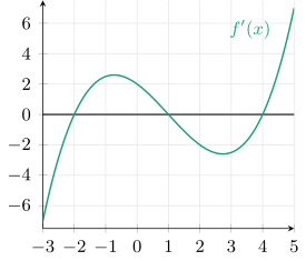
The graph below shows the derivative $f'(x)$ of a function $f(x)$ on $-3 \le x \le 5$ . For $-3 < x < 5$ , identify where $f$ is increasing or decreasing, the inputs of its local extrema, its concavity, and the inputs of its points of inflection.

ShowHide solution

The graph of $f'$ is below the $x$ -axis on $(-3, -2)$ and $(1, 4)$ and above the $x$ -axis on $(-2, 1)$ and $(4, 5)$ . Therefore, $f$ is decreasing on $(-3, -2)$ and $(1, 4)$ and increasing on $(-2, 1)$ and $(4, 5)$ . Because the derivative exists at every input of the graph, $f$ is continuous there. The function $f$ has local minima at $x = -2$ and $x = 4$ , where the sign of $f'$ changes from negative to positive. The function $f$ has a local maximum at $x = 1$ , where the sign changes from positive to negative.

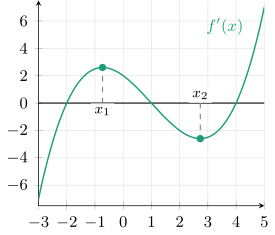
On the graph, $f'$ has a local maximum at an input $x_1$ between $-1$ and 0 and a local minimum at an input $x_2$ between 2 and 3. The graph of $f'$ rises on $(-3, x_1)$ and $(x_2, 5)$ and falls on $(x_1, x_2)$ . As a result, $f$ is concave up on $(-3, x_1)$ and $(x_2, 5)$ and concave down on $(x_1, x_2)$ . The function $f$ has points of inflection at the inputs $x_1$ and $x_2$ , because the concavity changes at each one.

The graph of $f'$ gives the inputs of the local extrema and the points of inflection of $f$ . To find the values of the local extrema and the heights of the points of inflection, use a formula or a graph of $f$ .

Lesson map