Lesson 27: The Derivative as a Function I

Objectives

Describe that in general, the derivative of a function is also a function.
Given a function, use R to approximate and plot its derivative.
Given the plot of a function, approximate its derivative graphically by hand.

1. Derivative Function

Objective. Describe that in general, the derivative of a function is also a function.

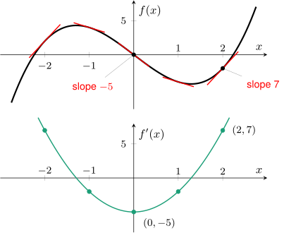
The top graph shows $f(x) = x^3 - 5x$ with its tangent line at five inputs, each slope estimated as in the Lesson 25 Notes, section 2. The bottom graph shows the slope of each tangent line as a height at the same input. The tangent line at $x = 2$ has slope 7, plotted as the point $(2, 7)$ . The tangent line at $x = 0$ has slope $-5$ , plotted as the point $(0, -5)$ . Every input of $f(x) = x^3 - 5x$ gives one slope, and plotting the slope at every input gives the green curve, the graph of the derivative function.

Definition 1 (Derivative function).

Let $f(x)$ be a function. The derivative function $f'(x)$ outputs the instantaneous rate of change of $f(x)$ for each input $x$ where that rate exists.

The number $f'(2)$ is not a derivative function. It is one output of $f'(x)$ , the instantaneous rate of change at the single input $x = 2$ , and the definition requires an output for each input $x$ where that rate exists.

Expression	Kind of object	Meaning
$f'(2)$	a number	the slope of the graph of $f(x)$ at $x = 2$
$f'(x)$	a function	assigns to each input $x$ the slope of the graph of $f(x)$ at $x$ , where the slope exists
$\frac{d}{dx}f(x)$	a function	the same function as $f'(x)$ , read “ $d$ $dx$ of $f$ of $x$ ”

Example 1

For the function

f(x) = x^3 - 5x,

the average rate of change on $[x, x + 0.001]$ approximates $f'(x)$ and takes these values at five inputs:

$x$	$-2$	$-1$	$0$	$1$	$2$
rate on $[x, x + 0.001]$	$6.994$	$-2.003$	$-5.000$	$-1.997$	$7.006$

Is the derivative of $f(x)$ a function?

ShowHide solution

By the definition of the derivative function, $f'(x)$ outputs the instantaneous rate of change of $f(x)$ for each input $x$ where that rate exists. The derivative of $f(x)$ is a function, because each input $x$ has exactly one instantaneous rate of change. The table gives estimates of $f'(x)$ at five inputs, and the rate changes with the input: $f'(0)$ is near $-5$ while $f'(2)$ is near $7$ . Each column of the table is a point $(x, \text{rate})$ near the green curve in the figure above, such as $(2, 7.006)$ near $(2, 7)$ .

Example 2

The height $H$ in meters of a ball thrown straight up, $t$ seconds after release, is

H(t) = 19.6t - 4.9t^{2}.

The average rate of change on $[t, t + 0.001]$ approximates $H'(t)$ and takes these values:

$t$	$0$	$1$	$2$	$3$	$4$
rate on $[t, t + 0.001]$	$19.595$	$9.795$	$-0.005$	$-9.805$	$-19.605$

Describe $H'(t)$ as a function: give its input and its output with units, and say what the table shows about the ball.

ShowHide solution

The derivative function $H'(t)$ takes as input a time $t$ in seconds and outputs the instantaneous rate of change of the height at that time, in meters per second. The derivative $H'(t)$ is a function of $t$ , because each time has exactly one instantaneous rate of change. The estimates decrease from about 19.595 meters per second at release to about $-19.605$ meters per second at $t = 4$ . The height increases at a decreasing rate until $t = 2$ . At $t = 2$ the estimate is $-0.005$ meters per second, a change in height of about 5 millimeters per second, against about 9.8 meters per second at $t = 1$ and at $t = 3$ . Therefore $H'(2) \approx 0$ , and the ball is at or very near the top of its flight at $t = 2$ . After $t = 2$ the rate is negative and the height decreases.

Lesson map

2. Approximating the Derivative in R

Objective. Given a function, use R to approximate and plot its derivative.

Approximating a derivative in R.

Define the function: f = makeFun(x^3 - 5*x ~ x).
Define the approximate derivative, the average rate of change from $x$ to $x + 0.001$ :
f_deriv = makeFun((f(x + 0.001) - f(x))/0.001 ~ x).
Evaluate f_deriv(a) to approximate $f'(a)$ .
Plot $f(x)$ with plotFun, then add the approximate derivative on top with plotFun(f_deriv(x) ~ x, add = TRUE).

Approximate derivative from f_change. After f_change from section 1 of the Lesson 25 Notes is defined, the line

f_deriv = makeFun(f_change(x, x + 0.001) ~ x)

also defines f_deriv, because f_change(x, x + 0.001) is the average rate of change on $[x, x + 0.001]$ .

Step size. The step is the width $h$ of the interval $[x, x + h]$ . For the functions in this course, shrinking a step of 0.001 down to about 0.000001 brings the average rate of change on $[x, x + h]$ closer to $f'(x)$ , or leaves it equal to $f'(x)$ when $f(x)$ is linear. Far smaller steps can make the estimate worse, because R rounds each output before subtracting.

For $f(x) = x^3 - 5x$ and a step $h$ , with $f(1) = 1 - 5 = -4$ , the average rate of change on $[1, 1 + h]$ simplifies to

\begin{aligned} \frac{f(1 + h) - f(1)}{h} &= \frac{(1 + h)^3 - 5(1 + h) - (-4)}{h} = \frac{1 + 3h + 3h^2 + h^3 - 5 - 5h + 4}{h}\\ &= \frac{-2h + 3h^2 + h^3}{h} = -2 + 3h + h^2, \end{aligned}

which approaches $f'(1) = -2$ as $h$ approaches $0$ . The table gives the estimate at three steps:

step	$0.8$	$0.3$	$0.001$
estimate of $f'(1)$	$1.04$	$-1.01$	$-1.996999$

Answers to three decimals. The estimate with step 0.001 can be wrong in the third decimal or earlier: at $x = 1$ it rounds to $-1.997$ , while $f'(1) = -2.000$ . For an answer to three decimals, shrink the step by a factor of 10 at a time with f_change until the stopping test in the Lesson 25 Notes, section 2, is met. When a problem gives the interval or the step, use that interval or step.

Order of definitions. The function f_deriv uses f. Evaluating f_deriv before f is defined gives an error:

> f_deriv(1)
Error in f(x + 0.001) : could not find function "f"

When f_deriv is defined from f_change, evaluating f_deriv before f_change is defined gives this error:

> f_deriv(1)
Error in f_change(x, x + 0.001) : could not find function "f_change"

Example 3

Approximate $f'(1)$ in R for the function

f(x) = x^3 - 5x

and plot the approximate derivative on top of $f(x)$ for $-3 \le x \le 3$ .

ShowHide solution

Define $f$ , the average rate of change f_change, and the approximate derivative f_deriv with step 0.001. Evaluate f_deriv(1), then shrink the step on each side of $x = 1$ with f_change until the stopping test is met. Used R.

f = makeFun(x^3 - 5*x ~ x)
f_change = makeFun((f(b) - f(a))/(b - a) ~ a & b)
f_deriv = makeFun((f(x + 0.001) - f(x))/0.001 ~ x)
f_deriv(1)
[1] -1.996999
f_change(1, 1.001)
[1] -1.996999
f_change(1, 1.0001)
[1] -1.9997
f_change(0.9999, 1)
[1] -2.0003
f_change(1, 1.00001)
[1] -1.99997
f_change(0.99999, 1)
[1] -2.00003

The call f_change(1, 1.001) returns the same $-1.996999$ as f_deriv(1), because both compute the average rate of change on $[1, 1.001]$ . At steps 0.0001 and 0.00001 the rates from both sides all round to $-2.000$ . The stopping test is met, and to three decimals

f'(1) \approx -2.000.

Plot $f(x)$ for $-3 \le x \le 3$ , then add the approximate derivative f_deriv on top. Used R.

plotFun(f(x) ~ x, xlim = range(-3, 3), ylim = range(-13, 23))
plotFun(f_deriv(x) ~ x, col = "darkgreen", add = TRUE)

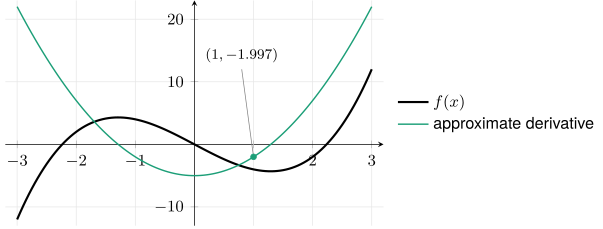
The first line plots $f(x)$ , and the second adds the plot of f_deriv in green. The green curve passes through $(1, -1.997)$ , whose height is the value f_deriv(1) returned, and its height at each input is approximately the slope of the black curve there.

Example 4

The function Weight models the average weight in grams of a male fetus, with input Week, the gestational age in weeks:

\text{Weight} = 781.9e^{0.1216(\text{Week} - 25)}.

Use R to approximate $\text{Weight}'(30)$ with step 0.001, and plot the approximate derivative for weeks 20 to 35.

ShowHide solution

Define Weight and the approximate derivative Weight_deriv with step 0.001, the average rate of change from Week to $\text{Week} + 0.001$ . Evaluate it at week 30 and at the ends of the plot, then plot it. Used R.

Weight = makeFun(781.9*exp(0.1216*(Week - 25)) ~ Week)
Weight_deriv = makeFun((Weight(Week + 0.001) - Weight(Week))/0.001 ~ Week)
Weight_deriv(30)
[1] 174.6474
Weight_deriv(c(20, 35))
[1]  51.76785 320.78443
plotFun(Weight_deriv(Week) ~ Week, xlim = range(20, 35))

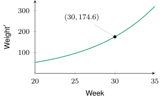
The line Weight_deriv(30) computes $\bigl(\text{Weight}(30.001) - \text{Weight}(30)\bigr)/0.001$ , which approximates $\text{Weight}'(30)$ . At step 0.001 the error of this estimate shows in the second decimal. Report the estimate to one decimal:

\text{Weight}'(30) \approx 174.6 \text{ grams per week}.

In week 30, the average male fetus’s weight is increasing at about 174.6 grams per week. The plot rises from about 51.8 grams per week at week 20 to about 320.8 grams per week at week 35. Because the approximate derivative increases, the weight increases at a greater rate each week.

Example 5

For the function

f(x) = x^3 - 5x,

use R to determine whether $f(1.5)$ is positive or negative, and whether $f(x)$ is increasing or decreasing at $x = 1.5$ .

ShowHide solution

Define $f$ and evaluate it at $x = 1.5$ . Used R.

f = makeFun(x^3 - 5*x ~ x)
f(1.5)
[1] -4.125

The value $f(1.5) = -4.125$ is negative.

The sign of $f'(1.5)$ determines whether $f(x)$ is increasing or decreasing. Approximate $f'(1.5)$ with the approximate derivative, as in Example 3, and check it with the average rates of change on each side of $x = 1.5$ at step 0.0001. Used R.

f_deriv = makeFun((f(x + 0.001) - f(x))/0.001 ~ x)
f_change = makeFun((f(b) - f(a))/(b - a) ~ a & b)
f_deriv(1.5)
[1] 1.754501
f_change(1.5, 1.5001)
[1] 1.75045
f_change(1.4999, 1.5)
[1] 1.74955

The rates from both sides of $x = 1.5$ are positive and close to the estimate 1.754501, far from 0. Therefore $f'(1.5)$ is positive, and $f(x)$ is increasing at $x = 1.5$ . Because the question asks only for the sign, the work stops without a three-decimal estimate or stopping test.

Lesson map

3. Sketching the Derivative from a Graph

Objective. Given the plot of a function, approximate its derivative graphically by hand.

The value $f'(a)$ is the slope of the tangent line to the graph of $f(x)$ at $x = a$ . The first four graphs show $f(x) = x^3 - 5x$ with one or two tangent lines. The last graph shows $g(x) = |x|$ , whose graph has a corner.

Positive derivative

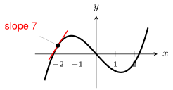
The graph rises left to right at $x = -2$ , and $f'(-2) \approx 7$ is positive.

Negative derivative

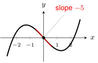
The graph falls left to right at $x = 0$ , and $f'(0) \approx -5$ is negative.

Zero derivative

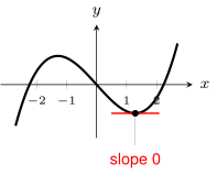
The graph has a valley near $x = 1.29$ , where the green approximate derivative of Example 3 crosses 0. The tangent line is horizontal there, and $f'(1.29) \approx 0$ .

Size of the derivative

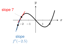
Because the blue tangent line at $x = -2.5$ is steeper than the red one at $x = -2$ , $f'(-2.5)$ is farther from zero than $f'(-2) \approx 7$ .

Undefined derivative

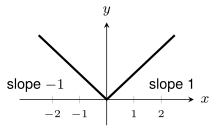
The graph of $g(x) = |x|$ has a corner at $x = 0$ with no single tangent line, and $g'(0)$ is undefined.

Sketching a derivative.

Mark each input where the graph of $f(x)$ has a horizontal tangent line. The derivative $f'(x)$ is zero there.
Draw $f'(x)$ above the $x$ -axis where $f(x)$ rises and below where $f(x)$ falls.
Estimate the slope of the graph of $f(x)$ at a few inputs and plot each slope as a point on the graph of $f'(x)$ . To estimate a slope, draw the tangent line at the input and divide its rise by its run between two points on it taken from the grid.
Join the points with a smooth curve. Leave a break at each corner.

Example 6

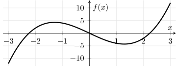
The graph of the function

f(x) = x^3 - 5x

has a peak near $x = -1.29$ and a valley near $x = 1.29$ . Sketch $f'(x)$ .

ShowHide solution

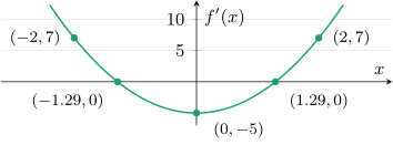
The derivative $f'(x)$ is zero at $x \approx -1.29$ and $x \approx 1.29$ , because the tangent line is horizontal at the peak and at the valley. The sign of $f'(x)$ is positive to the left of the peak and to the right of the valley, because $f(x)$ rises there. Between the peak and the valley the sign is negative, because $f(x)$ falls there.

Estimate three slopes, two from the graph and one by symmetry. Draw the tangent line at $x = 0$ on the grid. It passes through $(0, 0)$ and about $(1, -5)$ , and its slope is about

\frac{-5 - 0}{1 - 0} = -5.

Draw the tangent line at $x = 2$ . It passes through $(2, -2)$ and about $(3, 5)$ , and its slope is about

\frac{5 - (-2)}{3 - 2} = 7.

The slope at $x = -2$ is also about 7, because the graph is symmetric about the origin: the part of the graph near $x = -2$ is the part near $x = 2$ rotated half a turn about the origin. The slope falls from about 7 at $x = -2$ to about $-5$ at $x = 0$ and climbs back to about 7 at $x = 2$ , and by the same symmetry the slopes at $x = -a$ and $x = a$ match. Therefore, the sketch of $f'(x)$ is a U-shaped curve, symmetric about the vertical axis, with its lowest point near $(0, -5)$ , and the curve crosses the $x$ -axis at the peak and the valley inputs.

Example 7

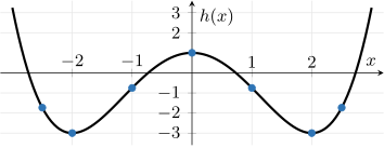
For the graph of $h(x)$ , determine where $h'(x)$ is zero, positive, and negative among the inputs

x = -2.5,\ -2,\ -1,\ 0,\ 1,\ 2,\ 2.5.

ShowHide solution

The derivative $h'(x)$ is zero at $x = -2$ , $0$ , and $2$ , because the graph has a valley, a peak, and a valley there.
The derivative $h'(x)$ is positive at $x = -1$ and $x = 2.5$ , because $h(x)$ rises there.
The derivative $h'(x)$ is negative at $x = -2.5$ and $x = 1$ , because $h(x)$ falls there.

Example 8

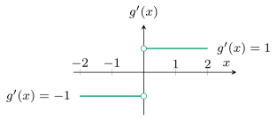
Sketch the derivative of

g(x) = |x|.

ShowHide solution

For $x < 0$ , $g'(x)$ equals $-1$ , because the graph of $g(x)$ there is a line of slope $-1$ . For $x > 0$ , $g'(x)$ equals $1$ , because the graph there is a line of slope $1$ .

At the corner $x = 0$ , the slope is $-1$ on the left and $1$ on the right. Because these two slopes differ, the graph has no single tangent line at $x = 0$ , and $g'(0)$ is undefined.

The sketch is a horizontal line at $-1$ for $x < 0$ and a horizontal line at $1$ for $x > 0$ , with a break at $x = 0$ . The open dots at $(0, -1)$ and $(0, 1)$ mark that $g'(0)$ is undefined.

Lesson map