Compute a Taylor polynomial of a given degree, centered at a given input, by hand and in R; understand that a linear approximation is a degree-one Taylor polynomial.
Understand how a Taylor polynomial uses derivatives to match certain behaviors of a function at a given input (value, slope, concavity, etc.).
Use a Taylor polynomial to estimate a function value at a given input, and compute the error, by hand and in R.
Understand how the degree and the distance from the “center” affect accuracy.
Objective. Compute a Taylor polynomial of a given degree, centered at a given input, by hand and in R; understand that a linear approximation is a degree-one Taylor polynomial.
For a whole number n, the notation f(n) means the nth derivative of f, with f(0)=f. The number n! (“n factorial”) is the product n⋅(n−1)⋯2⋅1, with 0!=1 and 1!=1. For example, 2!=2, 3!=6, and 4!=24.
Definition 1 (Taylor polynomial).
Let f have n derivatives at x=a. The degree n Taylor polynomial of f centered at x=a is the polynomial Tn of degree at most n whose value and first n derivatives at x=a match those of f:
The function f(x)=∣x∣ has no degree 1 Taylor polynomial centered at x=0, because the definition requires one derivative at x=0 and f′(0) does not exist. The average rates of change of ∣x∣ near 0 are 1 from the right and −1 from the left (Lesson 25 section 2).
Definition 2 (Center).
The center of Tn is the input a at which f and every derivative in Tn are evaluated.
In T1(x)=f(4)+f′(4)(x−4) evaluated at x=4.2, the input 4.2 is not the center, because f and its derivative are evaluated at 4 and 4.2 enters only through the factor x−4.
A Taylor polynomial centered at x=0 is also called a Maclaurin polynomial.
The degree 1 Taylor polynomial is the linear approximation of Lesson 30 section 1:
T1(x)=f(a)+f′(a)(x−a)=L(x).
To compute the degree n Taylor polynomial Tn of f centered at x=a by hand:
Take the derivatives of f up to the nth.
Evaluate f and each derivative at the center a.
For each k from 0 to n, divide the kth derivative’s value by k! and multiply by (x−a)k.
Add the n+1 terms.
Example 1
Find the degree 3 Taylor polynomial centered at x=0 of
f(x)=ex.
ShowHide solution
By the definition of a Taylor polynomial with n=3 and a=0, the degree 3 Taylor polynomial centered at x=0 is
T3(x)=f(0)+f′(0)x+2!f′′(0)x2+3!f′′′(0)x3.
Every derivative of ex is ex. By the definition of center, evaluate f and its first three derivatives at a=0:
f(0)=f′(0)=f′′(0)=f′′′(0)=e0=1.
Substitute the four values into the formula for T3:
T3(x)=1+1⋅x+2!1x2+3!1x3=1+x+2x2+6x3.
Example 2
Find the degree 1 and degree 2 Taylor polynomials centered at x=4 of
f(x)=x.
ShowHide solution
The degree 2 Taylor polynomial centered at x=4 is
T2(x)=f(4)+f′(4)(x−4)+2!f′′(4)(x−4)2,
and T1 is its first two terms. With f(x)=x1/2, f′(x)=21x−1/2, and f′′(x)=−41x−3/2, evaluate at the center:
Find the degree 2 Taylor polynomial centered at x=0 of
f(x)=e2x.
ShowHide solution
By the chain rule, f′(x)=2e2x and f′′(x)=4e2x. Evaluate at the center:
f(0)=e0=1,f′(0)=2e0=2,f′′(0)=4e0=4.
Substitute the three values into the formula for T2:
T2(x)=1+2x+2!4x2=1+2x+2x2.
Taylor polynomials in R. The command D(f(x) ~ x) returns the derivative, and D(f(x) ~ x & x) returns the second derivative (Lesson 29 section 5). Each added & x gives one more derivative: the third derivative is D(f(x) ~ x & x & x). The command factorial(k) returns k!. Build the Taylor polynomial with makeFun from the derivative values.
Example 5
Find the degree 3 Taylor polynomial centered at x=0 of
f(x)=ex
in R, and plot it with f.
ShowHide solution
Define f and its first three derivatives, and evaluate each at the center 0. Used R.
f = makeFun(exp(x) ~ x)df = D(f(x) ~ x)d2f = D(f(x) ~ x & x)d3f = D(f(x) ~ x & x & x)c(f(0), df(0), d2f(0), d3f(0))[1] 1 1 1 1
Build T3 from the four values with makeFun, and plot it in orange over the graph of f.
The R steps are the hand steps of Example 1. The line c(f(0), df(0), d2f(0), d3f(0)) prints f(0), f′(0), f′′(0), and f′′′(0). In the definition of T3, the term d2f(0)/factorial(2)*(x - 0)^2 is R’s form of the term 2!f′′(0)(x−0)2. With the four values equal to 1, T3 is the polynomial T3(x)=1+x+2x2+6x3 of Example 1.
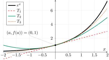
The figure in section 2 shows the same two graphs for −2≤x≤2: ex is the solid black curve, and T3 is the orange dotted curve. The figure also shows the degree 1 and degree 2 Taylor polynomials T1 and T2 of ex.
The center in makeFun. Write the center as a number. Inside makeFun, a letter such as a in place of 4 becomes a second input of the function:
> T1 = makeFun(f(4) + df(4)*(x - a) ~ x)> T1(4.2)Error in T1(4.2) : argument "a" is missing, with no default
Objective. Understand how a Taylor polynomial uses derivatives to match certain behaviors of a function at a given input (value, slope, concavity, etc.).
Theorem 3 (Matching at the center).
Let f have n derivatives at x=a. At the center x=a, the Taylor polynomial Tn has the same value as f and the same first n derivatives:
The table lists the behavior that Tn and f share at a under each matched condition.
Condition at the center
Behavior matched
Shared by Tn and f at a
Tn(a)=f(a)
value
both graphs pass through (a,f(a))
Tn′(a)=f′(a)>0
slope
both increasing at a
Tn′(a)=f′(a)<0
slope
both decreasing at a
Tn′′(a)=f′′(a)>0
concavity
both concave up at a
Tn′′(a)=f′′(a)<0
concavity
both concave down at a
The slope rows apply when n≥1, and the concavity rows apply when n≥2.
The graph of T1 is the tangent line to the graph of f at (a,f(a)), because T1 matches value and slope. When f′′(a)=0, the graph of T2 has the same concavity as the graph of f at x=a, because T2 also matches the second derivative. The polynomial Tn+1 matches one more derivative than Tn.
The figure shows ex with its degree 1, 2, and 3 Taylor polynomials centered at x=0; the degree 3 polynomial is the T3 of Example 1.
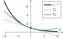
The function f(x)=e−x shows the decreasing case. Its derivatives f′(x)=−e−x and f′′(x)=e−x give f(0)=1, f′(0)=−1<0, and f′′(0)=1>0. The Taylor polynomials centered at x=0 are
T1(x)=1−x,T2(x)=1−x+2x2.
Both graphs fall through (0,1) with e−x, and T2 is concave up there like e−x.
Factorial coefficients. Let A be the coefficient of (x−a)k in Tn. The kth derivative of A(x−a)k is k!A, and each of the remaining terms of Tn has kth derivative 0 at x=a. For a term of lower degree, the kth derivative is 0. For a term of higher degree, the kth derivative still has a factor x−a, which is 0 at x=a. As a result, Tn(k)(a)=k!A, and matching f(k)(a) requires k!A=f(k)(a). The coefficient of (x−a)k is therefore k!f(k)(a).
Example 6
The degree 2 Taylor polynomial of a function f centered at x=2 is
T2(x)=5−3(x−2)+4(x−2)2.
Find f(2), f′(2), and f′′(2). Determine whether f is increasing or decreasing at x=2, and whether it is concave up or concave down there.
ShowHide solution
By the definition of a Taylor polynomial, the coefficient of (x−2)k is k!f(k)(2). The constant term is f(2)=5, and the coefficient of x−2 is f′(2)=−3. Since the coefficient of (x−2)2 is 2!f′′(2)=4,
f′′(2)=2!⋅4=8.
The function f is decreasing at x=2, because f′(2)<0. It is concave up there, because f′′(2)>0.
Example 7
Find the degree 4 Taylor polynomial centered at x=0 of
f(x)=cosx.
Then explain why it has no odd powers of x.
ShowHide solution
The derivatives of cosx are f′(x)=−sinx, f′′(x)=−cosx, f′′′(x)=sinx, and f(4)(x)=cosx. Evaluate f and its first four derivatives at the center:
Substitute the five values into the formula for T4:
T4(x)=1+0x+2!−1x2+3!0x3+4!1x4=1−2x2+24x4.
The odd powers drop out because the odd-order derivatives f′(0) and f′′′(0) are both 0 at the center.
Example 8
Find the degree 2 Taylor polynomial centered at x=2π of
f(x)=sinx.
ShowHide solution
With f′(x)=cosx and f′′(x)=−sinx, evaluate f and its first two derivatives at the center, where sin2π=1 and cos2π=0:
f(2π)=1,f′(2π)=cos2π=0,f′′(2π)=−sin2π=−1.
Substitute the three values into the formula for T2:
T2(x)=1+0(x−2π)−2!1(x−2π)2=1−21(x−2π)2.
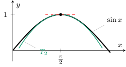
Since f′(2π)=0 and f′′(2π)<0, the function sinx has a maximum at x=2π. The polynomial T2 shares its value, slope, and concavity there. On the graph, T2 is a parabola that is concave down like sinx. It passes through the maximum point (2π,1) with a horizontal tangent line there.
The lines T1(4.2) and T2(4.2) compute the estimates, and each line with abs() computes the error ∣f(4.2)−Tn(4.2)∣ of the definition. The estimates and the errors match Example 9: T1(4.2)=2.05 with error about 0.000610, and T2(4.2)=2.049375 with error about 0.000015.
Scientific notation. R prints a very small number in scientific notation: 1.515319e-05 means 1.515319×10⁻⁵≈0.00001515.
Objective. Understand how the degree and the distance from the “center” affect accuracy.
An estimate is more accurate than another when its error is smaller. The table gives the error ∣eb−Tn(b)∣, rounded to four significant digits, for the Taylor polynomials of ex centered at x=0. Every derivative of ex is 1 at x=0. As a result, each entry is the distance between eb and Tn(b)=1+b+2!b2+⋯+n!bn.
∣eb−Tn(b)∣
b=0.1
b=0.5
b=1
b=2
T1
0.005171
0.1487
0.7183
4.389
T2
0.0001709
0.02372
0.2183
2.389
T3
0.000004251
0.002888
0.05162
1.056
T4
0.00000008474
0.0002838
0.009948
0.3891
Degree. Near the center, a higher-degree polynomial matches more derivatives of f at the center and often gives a smaller error. Each column of the ex table shows this.
An added term with coefficient 0 leaves the error unchanged. For cosx centered at x=0, the polynomials satisfy T3=T2, because f′′′(0)=0 (Example 7).
Far from the center, a higher degree can give a larger error. For lnx centered at x=1, the error at b=3 grows with each added degree. One more derivative of f(x)=lnx from Example 3 is f(4)(x)=−6x−4, with f(4)(1)=−6. The degree 4 term is therefore 4!−6(x−1)4=−4(x−1)4. At b=3, the factor x−1 is 2. Substitute 2 for x−1 in each polynomial:
With ln3=1.098612… from a calculator, the estimates and their errors are:
T1
T2
T3
T4
Tn(3)
2
0
2.667
−1.333
∣ln3−Tn(3)∣
0.9014
1.099
1.568
2.432
Distance from the center. At a fixed degree, an input farther from the center often gives a larger error, as each row of the ex table shows. The error of T4 grows from about 0.00000008474 at b=0.1 to about 0.3891 at b=2.
Example 12
For f(x)=lnx centered at x=1, the degree 3 Taylor polynomial is
T3(x)=(x−1)−2(x−1)2+3(x−1)3.
Estimate ln(1.1), ln(1.5), and ln(2) with T3, and determine which estimate is most accurate.
ShowHide solution
For each input b, substitute b into T3, then compute the error with the true value ln(b) from a calculator. For b=1.1,
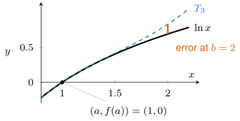
The estimate of ln(1.1) is the most accurate, because it has the smallest error. The input 1.1 is also the input closest to the center 1. On the graph, each error is the vertical gap between lnx and T3 at b: too small to see at b=1.1 and b=1.5, and visible at b=2.
Example 13
For f(x)=cosx centered at x=0, the degree 2 and degree 4 Taylor polynomials are
T2(x)=1−2x2,T4(x)=1−2x2+24x4.
Estimate cos(1) with each, and determine which degree gives the more accurate estimate.
ShowHide solution
For each polynomial, substitute b=1, then compute the error with the true value cos(1)=0.540302… from a calculator. For T2,
The degree 4 estimate is more accurate: its error 0.001364 is about 301 of the error 0.040302 of T2. The polynomial T4 also matches two more derivatives of cosx at the center than T2 does.