Lesson 29: Derivatives of Basic Functions

Objectives

Use the 1st and 2nd derivatives to characterize a function (increasing/decreasing, local extrema, concavity, inflection points).
Find derivatives of basic power functions using the power rule, by hand.
Find derivatives of basic modeling functions by hand (exponential, sinusoidal, logarithmic, etc.).
Compute derivatives of linear combinations using the constant, constant-multiple, and sum/difference rules.
In R, use D() to find the derivative of a function.

1. Characterizing a Function

Objective. Use the 1st and 2nd derivatives to characterize a function (increasing/decreasing, local extrema, concavity, inflection points).

Intervals of increase and decrease, local extrema, concavity, and points of inflection are read from the graphs of $f'$ and $f''$ in sections 3 and 4 of the Lesson 28 Notes. With formulas for $f'$ and $f''$ , the same intervals and points are found by algebra.

On an interval where $f'$ is defined, continuous, and never zero, $f'$ has one sign. As a result, the sign of $f'$ at a single test input in such an interval is the sign of $f'$ on the whole interval. The same is true of $f''$ .

Characterizing a function from $f'$ and $f''$ .

Find the inputs where $f'(x) = 0$ or where $f'(x)$ does not exist, and evaluate $f'$ at one test input in each interval those inputs mark off. The function $f$ is increasing on an interval with a positive test value and decreasing on an interval with a negative test value.
At each input where $f$ is continuous, report a local maximum where $f'$ changes from positive to negative and a local minimum where $f'$ changes from negative to positive. Substitute each such input into $f(x)$ for the value.
Find the inputs where $f''(x) = 0$ or where $f''(x)$ does not exist, and evaluate $f''$ at one test input in each interval those inputs mark off. The function $f$ is concave up on an interval with a positive test value and concave down on an interval with a negative test value.
Report a point of inflection $(c, f(c))$ at each input $c$ where the sign of $f''$ changes and $f$ is continuous.

Examples 1 and 2 give $f'$ and $f''$ in the stem. The rules for finding them from a formula for $f$ are in sections 2 to 4.

Example 1

The function

f(x) = x^3 - 3x^2 - 9x + 5

has first and second derivatives

f'(x) = 3(x + 1)(x - 3), \qquad f''(x) = 6(x - 1).

Determine where $f$ is increasing and decreasing, its local extrema, its concavity, and its points of inflection.

ShowHide solution

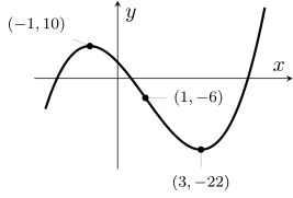
Because the derivative $f'$ exists at every input, $f$ is continuous everywhere. By the sign test for local extrema (Lesson 28 Notes, section 3), $f$ has a local extremum at each input where the sign of $f'$ changes. The factors of $f'$ are zero at $x = -1$ and $x = 3$ . Evaluate $f'$ at one input in each interval those inputs mark off:

f'(-2) = 3(-1)(-5) = 15 > 0, \qquad f'(0) = 3(1)(-3) = -9 < 0, \qquad f'(4) = 3(5)(1) = 15 > 0.

The function $f$ is increasing for $x < -1$ and for $x > 3$ , and decreasing for $-1 < x < 3$ . Because $f'$ changes from positive to negative at $x = -1$ and from negative to positive at $x = 3$ , $f$ has a local maximum at $x = -1$ and a local minimum at $x = 3$ . Substitute each input into $f(x)$ for the values:

\begin{align*} f(-1) &= (-1)^3 - 3(-1)^2 - 9(-1) + 5 = -1 - 3 + 9 + 5 = 10,\\ f(3) &= 3^3 - 3(3)^2 - 9(3) + 5 = 27 - 27 - 27 + 5 = -22. \end{align*}

The second derivative is zero at $x = 1$ . Evaluate $f''$ at one input on each side:

f''(0) = 6(0 - 1) = -6 < 0, \qquad f''(2) = 6(2 - 1) = 6 > 0.

The function $f$ is concave down for $x < 1$ and concave up for $x > 1$ . Because $f''$ changes sign at $x = 1$ , the point $(1, f(1))$ is a point of inflection, with

f(1) = 1^3 - 3(1)^2 - 9(1) + 5 = 1 - 3 - 9 + 5 = -6.

On the graph of $f$ , the local maximum $f(-1) = 10$ is the height of the peak at $(-1, 10)$ , and the local minimum $f(3) = -22$ is the height of the valley at $(3, -22)$ . At the point of inflection $(1, -6)$ , the graph changes from concave down to concave up.

Example 2

The function

g(x) = x^4 - 4x^3

has first and second derivatives

g'(x) = 4x^2(x - 3), \qquad g''(x) = 12x(x - 2).

Determine where $g$ is increasing and decreasing, its local extrema, its concavity, and its points of inflection.

ShowHide solution

The factors of $g'$ are zero at $x = 0$ and $x = 3$ . Evaluate $g'$ at one input in each interval those inputs mark off:

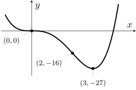
g'(-1) = 4(1)(-4) = -16 < 0, \qquad g'(1) = 4(1)(-2) = -8 < 0, \qquad g'(4) = 4(16)(1) = 64 > 0.

Thus, $g$ is decreasing for $x < 0$ and for $0 < x < 3$ , and increasing for $x > 3$ . The polynomial $g$ is continuous everywhere. Because $g'$ is negative on both sides of $x = 0$ , $g$ has no local extremum at $x = 0$ . The sign of $g'$ changes from negative to positive at $x = 3$ . By the sign test for local extrema, $g$ has a local minimum there:

g(3) = 3^4 - 4(3)^3 = 81 - 108 = -27.

The factors of $g''$ are zero at $x = 0$ and $x = 2$ . Evaluate $g''$ at one input in each interval:

g''(-1) = 12(-1)(-3) = 36 > 0, \qquad g''(1) = 12(1)(-1) = -12 < 0, \qquad g''(3) = 12(3)(1) = 36 > 0.

The function $g$ is concave up for $x < 0$ and for $x > 2$ , and concave down for $0 < x < 2$ . The concavity changes at both inputs, and the points of inflection are $(0, g(0))$ and $(2, g(2))$ , with

g(0) = 0^4 - 4(0)^3 = 0, \qquad g(2) = 2^4 - 4(2)^3 = 16 - 32 = -16.

On the graph of $g$ , the tangent line at $(0, 0)$ is horizontal, yet $g$ keeps decreasing to the local minimum $g(3) = -27$ at $(3, -27)$ . The concavity changes at $(0, 0)$ and $(2, -16)$ .

Lesson map

2. The Power Rule

Objective. Find derivatives of basic power functions using the power rule, by hand.

Rule 1 (Constant rule).

For every real number $c$ , the derivative of the constant function $c$ is 0,

\frac{d}{dx}[c] = 0.

For constants $m$ and $b$ , the derivative of the linear function $mx + b$ is its slope, $\frac{d}{dx}[mx + b] = m$ , because the tangent line to a line at every input is the line itself.

Rule 2 (Power rule).

For every real number $n$ ,

\frac{d}{dx}[x^n] = nx^{n-1}

for every $x$ with $x > 0$ , for every $x$ when $n$ is a positive integer, and for every $x$ with $x \neq 0$ when $n$ is a negative integer.

Why it works: the power rule for a positive integer

n

For a positive integer $n$ , every pair of numbers $a$ and $b$ satisfies the factoring

a^n - b^n = (a - b)\left(a^{n-1} + a^{n-2}b + \dots + b^{n-1}\right).

Substitute $a = x + h$ and $b = x$ into the factoring. The quotient in the limit definition of the derivative (Lesson 26 Notes, section 4) becomes

\frac{(x + h)^n - x^n}{h} = (x + h)^{n-1} + (x + h)^{n-2}x + \dots + x^{n-1}

for $h \neq 0$ . The right side has $n$ terms, and each approaches $x^{n-1}$ as $h \to 0$ . The limit is therefore $nx^{n-1}$ . For other $n$ the rule can fail at $x = 0$ . For example, the function $\sqrt{x} = x^{1/2}$ has no derivative at 0, and the formula $\tfrac{1}{2}x^{-1/2}$ gives no value there.

Rewriting as a power. The power rule applies to $x^n$ only. Before the power rule is applied, a root becomes a power with a fractional exponent, and 1 over a power becomes a power with a negative exponent. For integers $p$ and $q$ with $q > 0$ , and every real number $n$ ,

\sqrt[q]{x^p} = x^{p/q} \ \text{for } x > 0, \qquad \frac{1}{x^n} = x^{-n} \ \text{for } x > 0.

When $n$ is an integer, the second rewrite is true for every $x$ with $x \neq 0$ . Combine a product or quotient of powers of $x$ into one power first: add the exponents of factors that multiply, and subtract the exponent of a factor that divides. The power rule applies to the single power that results.

Example 3

Find the derivatives:

\frac{1}{x^5}, \qquad \sqrt{x^3}, \qquad \frac{1}{\sqrt[5]{x^3}}.

ShowHide solution

Rewrite each function as a power $x^n$ , then apply the power rule $\frac{d}{dx}[x^n] = nx^{n-1}$ .

The first function, 1 over a power, becomes a power with a negative exponent, $\frac{1}{x^5} = x^{-5}$ :

\frac{d}{dx}\left[x^{-5}\right] = -5x^{-5 - 1} = -5x^{-6} = -\frac{5}{x^6}

for every $x$ with $x \neq 0$ . The rewrite is true for these inputs because the exponent $-5$ is an integer.

The root in the second function becomes a power with a fractional exponent, $\sqrt{x^3} = x^{3/2}$ :

\frac{d}{dx}\left[x^{3/2}\right] = \frac{3}{2}x^{3/2 - 1} = \frac{3}{2}x^{1/2}

for every $x$ with $x > 0$ . The rewriting lead gives the rewrite for these inputs.

Apply both rewrites to the third function. The root is $\sqrt[5]{x^3} = x^{3/5}$ , and 1 over that power becomes a power with a negative exponent, $\frac{1}{\sqrt[5]{x^3}} = x^{-3/5}$ :

\frac{d}{dx}\left[x^{-3/5}\right] = -\frac{3}{5}x^{-3/5 - 1} = -\frac{3}{5}x^{-8/5}

for every $x$ with $x > 0$ . The rewriting lead gives both rewrites for these inputs.

Example 4

Find the derivative:

\frac{x^4\sqrt[3]{x}}{x^2}.

ShowHide solution

Write the root as $\sqrt[3]{x} = x^{1/3}$ and combine the exponents into one power:

\frac{x^4\sqrt[3]{x}}{x^2} = \frac{x^4 x^{1/3}}{x^2} = x^{4 + 1/3 - 2} = x^{7/3}.

Apply the power rule:

\frac{d}{dx}\left[x^{7/3}\right] = \frac{7}{3}x^{7/3 - 1} = \frac{7}{3}x^{4/3}

for every $x$ with $x > 0$ . The rewriting lead gives the rewrites for these inputs.

The words estimate and find. “Estimate $f'(a)$ ” asks for the average rate of change over a short interval. “Find” or “compute” $f'(a)$ asks for the value of the derivative itself, from a derivative rule by hand or from D() in R.

Example 5

For the function

f(x) = \frac{1}{x^3},

estimate $f'(2)$ with an interval of width 0.001, then compute $f'(2)$ exactly.

ShowHide solution

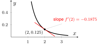
Estimate $f'(2)$ with the average rate of change from 2 to 2.001:

f'(2) \approx \frac{f(2.001) - f(2)}{0.001} = \frac{\frac{1}{2.001^3} - \frac{1}{2^3}}{0.001} \approx \frac{0.124813 - 0.125}{0.001} \approx -0.187.

Rewrite $f(x) = x^{-3}$ and apply the power rule for the exact value:

f'(x) = -3x^{-3 - 1} = -3x^{-4} \quad\text{so}\quad f'(2) = -3(2)^{-4} = -\frac{3}{16} = -0.1875.

The estimate is within 0.001 of the exact value. The exact value is the slope of the tangent line to the graph of $f$ at $(2, f(2)) = (2, 0.125)$ , and the estimate is the slope of a secant line close to it.

Lesson map

3. Basic Modeling Functions

Objective. Find derivatives of basic modeling functions by hand (exponential, sinusoidal, logarithmic, etc.).

Definition 3 (Basic modeling functions).

The basic modeling functions are the simplest forms of the modeling functions. For constants $m$ , $b$ , and $n$ and a constant $a$ with $a > 0$ , they are

mx + b, \qquad x^n, \qquad e^x, \qquad a^x, \qquad \ln(x), \qquad \sin(x), \qquad \cos(x).

The function $e^x\sin(x)$ is not a basic modeling function, because it multiplies two basic modeling functions together and is none of the forms in the definition. Lesson 30 differentiates products.

The sine and cosine rules below hold for $x$ in radians, the textbook’s unit for angles.

Rule 4 (Derivatives of basic modeling functions).

For a constant $a$ with $a > 0$ and constants $m$ and $b$ , the basic modeling functions have these derivatives:

\begin{array}{ll} \text{Exponential rule:} & \frac{d}{dx}[e^x] = e^x, \qquad \frac{d}{dx}[a^x] = a^x\ln(a), \\[6pt] \text{Extended exponential rule:} & \frac{d}{dx}[e^{mx + b}] = me^{mx + b}, \\[6pt] \text{Logarithm rule:} & \frac{d}{dx}[\ln(x)] = \dfrac{1}{x} \text{ for } x > 0, \\[6pt] \text{Sine and cosine rules:} & \frac{d}{dx}[\sin(x)] = \cos(x), \qquad \frac{d}{dx}[\cos(x)] = -\sin(x). \end{array}

Linear exponent. The extended exponential rule applies when the exponent is linear in $x$ . Differentiating $e^{x^2}$ or $e^{\cos(x)}$ , where the exponent is not linear, takes the chain rule (Lesson 32).

Power or exponential. In a power function the variable is the base, as in $x^3$ , and the power rule applies. In an exponential function the variable is the exponent, as in $3^x$ , and the exponential rule $\frac{d}{dx}[a^x] = a^x\ln(a)$ applies. Thus $\frac{d}{dx}[x^3] = 3x^2$ and $\frac{d}{dx}[3^x] = 3^x\ln(3)$ .

Constant expressions. An expression with no $x$ in it, such as $\cos(4)$ , $\ln(6)$ , $e^2$ , or $\pi$ , is a constant with derivative 0.

Example 6

Find the derivatives:

7^x, \qquad x^7, \qquad e^{3x - 2}, \qquad \cos(x), \qquad \ln(2).

ShowHide solution

By the exponential rule, $\frac{d}{dx}[7^x] = 7^x\ln(7)$ .
By the power rule, $\frac{d}{dx}[x^7] = 7x^6$ .
By the extended exponential rule with $m = 3$ , $\frac{d}{dx}[e^{3x - 2}] = 3e^{3x - 2}$ .
By the cosine rule, $\frac{d}{dx}[\cos(x)] = -\sin(x)$ .
Because $\ln(2)$ is a constant, $\frac{d}{dx}[\ln(2)] = 0$ .

Example 7

Find each derivative and evaluate it at the given input:

\ln(x) \text{ at } x = 4, \qquad \sin(x) \text{ at } x = \frac{\pi}{3}, \qquad 2^x \text{ at } x = 3.

ShowHide solution

By the logarithm rule, $\frac{d}{dx}[\ln(x)] = \dfrac{1}{x}$ . At $x = 4$ the derivative is $\dfrac{1}{4} = 0.25$ .
By the sine rule, $\frac{d}{dx}[\sin(x)] = \cos(x)$ . At $x = \frac{\pi}{3}$ the derivative is $\cos\!\left(\frac{\pi}{3}\right) = 0.5$ .
By the exponential rule, $\frac{d}{dx}[2^x] = 2^x\ln(2)$ . At $x = 3$ the derivative is $2^3\ln(2) = 8\ln(2) \approx 5.545$ .

Example 8

Determine which of these functions are differentiated with the power rule:

x^4, \qquad 4^x, \qquad \frac{1}{x^4}, \qquad e^{4x}, \qquad \ln(x).

ShowHide solution

The functions $x^4$ and $1/x^4 = x^{-4}$ are differentiated with the power rule, because in each the variable is the base and the exponent is a constant. The function $4^x$ is differentiated with the exponential rule, because the variable is the exponent. The function $e^{4x}$ is differentiated with the extended exponential rule, because its exponent $4x$ is linear in $x$ . The function $\ln(x)$ is differentiated with the logarithm rule, because it is the natural logarithm.

Lesson map

4. Linear Combinations

Objective. Compute derivatives of linear combinations using the constant, constant-multiple, and sum/difference rules.

Rule 5 (Constant multiple rule).

For a real number $k$ and a differentiable function $f(x)$ ,

\frac{d}{dx}[k\,f(x)] = k\,f'(x).

Rule 6 (Sum and difference rules).

For differentiable functions $f(x)$ and $g(x)$ ,

\frac{d}{dx}[f(x) \pm g(x)] = f'(x) \pm g'(x).

Definition 7 (Linear combination).

A linear combination of functions is a sum of constant multiples of the functions, such as $3f(x) - 2g(x)$ .

The function $x^2\sin(x)$ is not a linear combination of $x^2$ and $\sin(x)$ , because it is a product of the two functions, and the definition allows only a sum of constant multiples. Products are differentiated in Lesson 30.

With the constant multiple rule and the sum and difference rules, a linear combination is differentiated one term at a time. A constant term has derivative 0 by the constant rule (section 2).

Example 9

Find $f'(x)$ :

f(x) = 5x^4 - \frac{3}{x} + 6\sin(x) + \cos(2) - 4\ln(x) + 2^x.

ShowHide solution

Rewrite $-3/x$ as $-3x^{-1}$ . By the definition of a linear combination, $f$ is a sum of constant multiples of $x^4$ , $x^{-1}$ , $\sin(x)$ , $\ln(x)$ , $2^x$ , and the constant function 1. The term $\cos(2)$ is a number times the constant function 1; the 3 in the Lesson 17 non-example $2\overline{\vphantom{b}u} + 3$ is a scalar with no vector. Differentiate term by term with the constant multiple rule, the sum and difference rules, the power, sine, logarithm, and exponential rules, and the constant rule for $\cos(2)$ :

\begin{align*} f'(x) &= 5(4x^3) - 3(-x^{-2}) + 6\cos(x) + 0 - 4\left(\frac{1}{x}\right) + 2^x\ln(2)\\ &= 20x^3 + \frac{3}{x^2} + 6\cos(x) - \frac{4}{x} + 2^x\ln(2). \end{align*}

Example 10

Name the rules needed to differentiate $h$ , then find $h'(x)$ :

h(x) = \frac{1}{4x^2} + e^x.

ShowHide solution

Rewrite the first term as a constant times a power:

\frac{1}{4x^2} = \frac{1}{4} \cdot \frac{1}{x^2} = \frac{1}{4}x^{-2}.

The rules needed are the constant multiple rule, the power rule, the sum and difference rules, and the exponential rule. Apply them term by term:

h'(x) = \frac{1}{4}\left(-2x^{-3}\right) + e^x = -\frac{1}{2}x^{-3} + e^x.

Example 11

Find the first four derivatives of the function

f(x) = x^3 - 5x.

ShowHide solution

Differentiate each derivative to get the next one:

f'(x) = 3x^2 - 5, \qquad f''(x) = 6x, \qquad f'''(x) = 6, \qquad f^{(4)}(x) = 0.

The third and fourth derivatives are written $f'''(x)$ and $f^{(4)}(x)$ , the $n$ th-derivative notation of the Lesson 28 Notes, section 2.

Example 12

For a constant $v_0$ in meters per second and a constant $p$ in meters, a projectile’s height in meters $t$ seconds after launch is

h(t) = -4.9t^2 + v_0t + p.

Find the velocity $h'(t)$ and the acceleration $h''(t)$ , the rate of change of the velocity, with units.

ShowHide solution

By the constant multiple rule and the power rule, $-4.9t^2$ has derivative $-4.9(2t) = -9.8t$ , and $v_0t$ has derivative $v_0(1) = v_0$ . The constant $p$ has derivative 0:

h'(t) = -9.8t + v_0.

Differentiate $h'$ the same way. The term $-9.8t$ has derivative $-9.8$ , and the constant $v_0$ has derivative 0:

h''(t) = -9.8.

The velocity $h'(t)$ is in meters per second, and the acceleration $h''(t)$ is in meters per second per second.

Lesson map

5. Derivatives in R

Objective. In R, use D() to find the derivative of a function.

The command D(formula ~ x) differentiates the left side of the tilde with respect to $x$ and returns the derivative as a function. The left side is either an expression in $x$ or a stored function written as f(x).

A derivative stored under a name such as df is evaluated and plotted the same way as a function from makeFun.

To find the second derivative, write the variable twice after the tilde, as in d2f = D(f(x) ~ x & x).

The natural logarithm and $e^x$ in R. The natural logarithm is log(x), and $e^x$ is exp(x). A call to ln() gives an error:

> ln(2)
Error in ln(2) : could not find function "ln"

When $e^x$ is typed as e^ x, R treats the letter e as a second input of the derivative. Evaluating the derivative at one input then gives an error:

> de = D(e^ x ~ x)
> de(1)
Error in de(1) : argument "e" is missing, with no default

Example 13

For the function

f(x) = x^3 - 5x,

find $f'(x)$ , $f'(0)$ , and $f''(1)$ in R.

ShowHide solution

Differentiate the expression with D() to see $f'(x)$ . Then store $f$ and its first and second derivatives, evaluate $f'$ at $x = 0$ , and evaluate $f''$ at $x = 1$ . Used R.

D(x^3 - 5*x ~ x)
function (x)
3 * x^2 - 5
f = makeFun(x^3 - 5*x ~ x)
df = D(f(x) ~ x)
df(0)
[1] -5
d2f = D(f(x) ~ x & x)
d2f(1)
[1] 6

R prints function (x) and then the body 3 * x^2 - 5, its spelling of $f'(x) = 3x^2 - 5$ . The calls df(0) and d2f(1) give $f'(0) = -5$ and $f''(1) = 6$ . As a check by hand, $f'(x) = 3x^2 - 5$ and $f''(x) = 6x$ give

f'(0) = 3(0)^2 - 5 = -5, \qquad f''(1) = 6(1) = 6.

Example 14

For the function

g(x) = 6\ln(x) - 3e^x,

find $g'(1)$ and $g''(1)$ by hand, and check both in R.

ShowHide solution

The constant multiple rule, the difference rule, the logarithm rule, and the exponential rule give

g'(x) = \frac{6}{x} - 3e^x \quad\text{so}\quad g'(1) = \frac{6}{1} - 3e^1 = 6 - 3e \approx -2.155.

Differentiating again, with $\frac{6}{x} = 6x^{-1}$ and the power rule, gives

g''(x) = -6x^{-2} - 3e^x = -\frac{6}{x^2} - 3e^x \quad\text{so}\quad g''(1) = -6 - 3e \approx -14.155.

Check both values in R. The command D() returns $g'$ and $g''$ as functions, and evaluating them at 1 gives the values to more digits. Used R.

g = makeFun(6*log(x) - 3*exp(x) ~ x)
dg = D(g(x) ~ x)
dg(1)
[1] -2.154845
d2g = D(g(x) ~ x & x)
d2g(1)
[1] -14.15485

R’s values agree with the hand values $g'(1) \approx -2.155$ and $g''(1) \approx -14.155$ .

Example 15

Find $q'(\pi)$ in R:

q(x) = \ln(5) + 3x^4 - e^x + \sin(x).

ShowHide solution

Differentiate $q$ with D() and evaluate the derivative at $\pi$ . Used R.

dq = D(log(5) + 3*x^4 - exp(x) + sin(x) ~ x)
dq(pi)
[1] 347.9346

Therefore $q'(\pi) \approx 347.935$ . As a check, the derivative by hand, $q'(x) = 12x^3 - e^x + \cos(x)$ , gives $12\pi^3 - e^{\pi} + \cos(\pi) \approx 347.935$ .

Lesson map