Lesson 38: Partial Derivatives II

Objectives

Using R, compute partial derivatives of a multivariable function.
Obtain higher-order partial derivatives by hand.
Use partial derivatives to obtain a linear approximation of a multivariable function at a point.

1. Partial Derivatives in R

Objective. Using R, compute partial derivatives of a multivariable function.

The R command D(f(x,y) ~ x) returns $f_x$ , the partial derivative of $f(x,y)$ with respect to the variable written immediately after the tilde, as a function of every input. The command D(f(x,y) ~ y) returns $f_y$ .

After dfx = D(f(x,y) ~ x), evaluate $f_x$ at $(1,2)$ with dfx(x = 1, y = 2), or with dfx(1, 2), which takes the values in the order $x$ , $y$ . A call with an input left out stops with an error:

> dfx(1)
Error in dfx(1) : argument "y" is missing, with no default

Example 1

Use R to compute $f_x$ and $f_y$ , then evaluate both at $(1, 2)$ :

f(x,y) = xy^2 + x^3.

ShowHide solution

Define $f$ with makeFun(), compute each first partial derivative with D(), and evaluate both partial derivatives at $(1,2)$ . Used R.

f = makeFun(x*y^2 + x^3 ~ x & y)
dfx = D(f(x,y) ~ x)
dfy = D(f(x,y) ~ y)
dfx(x = 1, y = 2)
[1] 7
dfy(x = 1, y = 2)
[1] 4

R returns $f_x(1,2) = 7$ and $f_y(1,2) = 4$ . As a check, the command dfx alone prints the formula R found, 3 * x^2 + y^2, which is $f_x(x,y) = 3x^2 + y^2$ from the derivative rules. The command dfy alone prints 2 * x * y, which is $f_y(x,y) = 2xy$ .

Example 2

Use R to compute $f_x(1,2)$ and $f_y(1,2)$ :

f(x,y) = \cos(xy) + x^2y^3.

ShowHide solution

Define $f$ , compute $f_x$ and $f_y$ with D(), and evaluate both at $(1,2)$ . Used R.

f = makeFun(cos(x*y) + x^2*y^3 ~ x & y)
dfx = D(f(x,y) ~ x)
dfy = D(f(x,y) ~ y)
dfx(x = 1, y = 2)
[1] 14.18141
dfy(x = 1, y = 2)
[1] 11.0907

R returns $f_x(1,2) \approx 14.181$ and $f_y(1,2) \approx 11.091$ .

To check by hand, treat $y$ as a constant and apply the chain rule to $\cos(xy)$ :

\begin{align*} f_x &= \frac{\partial}{\partial x}\left[\cos(xy) + x^2y^3\right] = -y\sin(xy) + 2xy^3,\\ f_x(1,2) &= -2\sin(2) + 2(1)(2)^3 = 16 - 2\sin(2) \approx 14.181. \end{align*}

The hand value agrees with the value from R.

Example 3

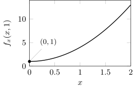
For $f(x,y) = xy^2 + x^3$ , plot $f_x$ in R for $0 \le x \le 2$ with $y$ held at 1, and determine whether $f$ increases or decreases in $x$ when $y = 1$ .

ShowHide solution

Define $f$ and $f_x$ in R, then plot $f_x$ with $y$ held at 1. Used R.

f = makeFun(x*y^2 + x^3 ~ x & y)

dfx = D(f(x,y) ~ x)

plotFun(dfx(x, y = 1) ~ x, xlim = range(0, 2))

In the formula dfx(x, y = 1) ~ x, the argument y = 1 fixes $y$ at 1, and ~ x puts $x$ on the horizontal axis.

By hand, treat $y$ as a constant, differentiate, and then set $y = 1$ :

\begin{align*} f_x &= \frac{\partial}{\partial x}\left[xy^2 + x^3\right] = y^2 + 3x^2,\\ f_x(x,1) &= 1^2 + 3x^2 = 1 + 3x^2. \end{align*}

Because $3x^2 \ge 0$ , the partial derivative satisfies $f_x(x,1) \ge 1$ for every $x$ , and the plot stays above the $x$ -axis. The lowest point of the plot is $(0, 1)$ , because $3x^2 = 0$ only at $x = 0$ , where $f_x(0,1) = 1$ . The function $f$ increases in $x$ when $y = 1$ , because a positive rate of change means an increasing output (Lesson 25 Notes, section 4). As a check, the one-input function $f(x,1) = x + x^3$ rises from $f(0,1) = 0$ to $f(2,1) = 10$ .

Lesson map

2. Higher-Order Partial Derivatives

Objective. Obtain higher-order partial derivatives by hand.

Definition 1 (Higher-order partial derivatives).

A second partial derivative is a partial derivative of a first partial derivative. A higher-order partial derivative is a partial derivative of a partial derivative, and the second partial derivatives are the higher-order partial derivatives of order 2. A two-variable function $f(x,y)$ has four second partial derivatives:

f_{xx} = [f_x]_x, \qquad f_{xy} = [f_x]_y, \qquad f_{yx} = [f_y]_x, \qquad f_{yy} = [f_y]_y.

The notation $[f_x]_y$ means the partial derivative of $f_x$ with respect to $y$ . The order of a partial derivative is the number of differentiations it takes: $f_x$ has order 1, $f_{xy}$ has order 2, and $f_{xxy}$ has order 3.

The first partial derivative $f_x$ is neither a second partial derivative nor a higher-order partial derivative, because it is a partial derivative of $f$ itself, and $f$ is not a partial derivative. Both definitions require a partial derivative of a partial derivative, such as $f_{xx} = [f_x]_x$ or $f_{xxy} = [f_{xx}]_y$ .

As in the textbook, each function in the examples is assumed to have partial derivatives of every order at the points where they are computed.

A mixed partial is a higher-order partial derivative that involves differentiating with respect to different input variables, such as $f_{xy}$ and $f_{yx}$ .

Order of differentiation. In subscript notation, find $f_{xy}$ by differentiating with respect to $x$ first and then with respect to $y$ . In Leibniz notation, differentiate first with respect to the rightmost variable in the denominator and work leftward:

\frac{\partial^2 f}{\partial y\,\partial x} = f_{xy}.

The exponent on $\partial$ in the numerator is the order. For repeated differentiation with respect to one variable, write an exponent on that variable in the denominator:

\frac{\partial^2 f}{\partial x^2} = f_{xx}, \qquad \frac{\partial^2 f}{\partial y^2} = f_{yy}.

A multivariable function $f(x,y)$ is smooth on an open region if and only if $f(x,y)$ has continuous partials of all orders at every point of that region.

The common modeling functions are smooth on every open region inside their domains.

Theorem 2 (Clairaut’s theorem).

If $f(x,y)$ is smooth on an open region, then $f_{xy}(x,y) = f_{yx}(x,y)$ at every point of that region.

Example 4

For a function $f(x,y,z)$ , list the order of differentiation for each partial derivative:

f_{yzx}, \qquad\qquad \frac{\partial^3 f}{\partial z\,\partial y\,\partial x}.

ShowHide solution

In $f_{yzx}$ , the order is $y$ , then $z$ , then $x$ , because subscripts are read left to right. In the partial derivative written in Leibniz notation, the order is $x$ , then $y$ , then $z$ , because the Leibniz denominator is read from the rightmost variable leftward. In subscript notation, that partial derivative is $f_{xyz}$ .

Example 5

Compute all second partial derivatives of

f(x,y) = xy^2 + x^3.

ShowHide solution

By the definition of higher-order partial derivatives, each second partial derivative is a partial derivative of a first one. Compute $f_x$ and differentiate it with respect to $x$ and to $y$ , then do the same with $f_y$ .

Differentiate $f$ with respect to $x$ , treating $y$ as a constant:

f_x = \frac{\partial}{\partial x}\left[xy^2 + x^3\right] = y^2 + 3x^2.

Differentiate $f_x$ with respect to $x$ and then with respect to $y$ :

f_{xx} = \frac{\partial}{\partial x}\left[y^2 + 3x^2\right] = 6x, \qquad f_{xy} = \frac{\partial}{\partial y}\left[y^2 + 3x^2\right] = 2y.

Differentiate $f$ with respect to $y$ , treating $x$ as a constant:

f_y = \frac{\partial}{\partial y}\left[xy^2 + x^3\right] = x(2y) + 0 = 2xy.

Differentiate $f_y$ with respect to $x$ and then with respect to $y$ :

f_{yx} = \frac{\partial}{\partial x}\left[2xy\right] = 2y, \qquad f_{yy} = \frac{\partial}{\partial y}\left[2xy\right] = 2x.

The mixed partials $f_{xy}$ and $f_{yx}$ both equal $2y$ . Clairaut’s theorem predicts this equality, because a polynomial is smooth everywhere.

Example 6

Compute all second partial derivatives of

g(x,y) = x^4\sin(y).

ShowHide solution

As in Example 5, start with $g_x$ , where the factor $\sin(y)$ is a constant multiple, and differentiate it with respect to $x$ and then $y$ :

\begin{align*} g_x &= \frac{\partial}{\partial x}\bigl[x^4\sin(y)\bigr] = 4x^3\sin(y),\\ g_{xx} &= \frac{\partial}{\partial x}\bigl[4x^3\sin(y)\bigr] = 12x^2\sin(y), \qquad g_{xy} = \frac{\partial}{\partial y}\bigl[4x^3\sin(y)\bigr] = 4x^3\cos(y). \end{align*}

Do the same with $g_y$ , where the factor $x^4$ is a constant multiple:

\begin{align*} g_y &= \frac{\partial}{\partial y}\bigl[x^4\sin(y)\bigr] = x^4\cos(y),\\ g_{yx} &= \frac{\partial}{\partial x}\bigl[x^4\cos(y)\bigr] = 4x^3\cos(y), \qquad g_{yy} = \frac{\partial}{\partial y}\bigl[x^4\cos(y)\bigr] = -x^4\sin(y). \end{align*}

The mixed partials $g_{xy}$ and $g_{yx}$ are equal, as Clairaut’s theorem states for the smooth function $x^4\sin(y)$ .

Example 7

Compute all second partial derivatives of the function below, then compute the third partial derivative $\dfrac{\partial^3 q}{\partial y\,\partial x^2}$ :

q(x,y) = x^3e^{4y}.

ShowHide solution

As in Example 5, start with $q_x$ , where the factor $e^{4y}$ is a constant multiple, and differentiate it with respect to $x$ and then $y$ . The computation of $q_{xy}$ uses $\frac{\partial}{\partial y}\bigl[e^{4y}\bigr] = 4e^{4y}$ from the chain rule:

\begin{align*} q_x &= \frac{\partial}{\partial x}\bigl[x^3e^{4y}\bigr] = 3x^2e^{4y},\\ q_{xx} &= \frac{\partial}{\partial x}\bigl[3x^2e^{4y}\bigr] = 6xe^{4y}, \qquad q_{xy} = \frac{\partial}{\partial y}\bigl[3x^2e^{4y}\bigr] = 3x^2 \cdot 4e^{4y} = 12x^2e^{4y}. \end{align*}

Do the same with $q_y$ , where the factor $x^3$ is a constant multiple:

\begin{align*} q_y &= \frac{\partial}{\partial y}\bigl[x^3e^{4y}\bigr] = x^3 \cdot 4e^{4y} = 4x^3e^{4y},\\ q_{yx} &= \frac{\partial}{\partial x}\bigl[4x^3e^{4y}\bigr] = 12x^2e^{4y}, \qquad q_{yy} = \frac{\partial}{\partial y}\bigl[4x^3e^{4y}\bigr] = 4x^3 \cdot 4e^{4y} = 16x^3e^{4y}. \end{align*}

The coefficient 16 of $q_{yy}$ is $4 \cdot 4$ , one factor of 4 from each differentiation with respect to $y$ .

The Leibniz denominator $\partial y\,\partial x^2$ read from the right gives the order $x$ , $x$ , then $y$ . The third partial derivative is $q_{xxy}$ . Differentiate $q_{xx}$ with respect to $y$ :

q_{xxy} = \frac{\partial}{\partial y}\bigl[6xe^{4y}\bigr] = 6x \cdot 4e^{4y} = 24xe^{4y}.

Higher-order partial derivatives in R. List the variables of differentiation in order after the tilde, separated by &. The call D(f(x,y) ~ x & y) computes $f_{xy}$ . The call D(f(x,y) ~ x & x) computes $f_{xx}$ .

Example 8

The second partial derivatives of $g(x,y) = x^4\sin(y)$ are

g_{xx} = 12x^2\sin(y), \qquad g_{xy} = g_{yx} = 4x^3\cos(y), \qquad g_{yy} = -x^4\sin(y).

Use R to check them at the point $(2, 1)$ .

ShowHide solution

Define $g$ , compute the four second partial derivatives with D() by listing the variables of differentiation in order, and evaluate each at $(2,1)$ . Used R.

g = makeFun(x^4*sin(y) ~ x & y)
dgxx = D(g(x,y) ~ x & x)
dgxy = D(g(x,y) ~ x & y)
dgyx = D(g(x,y) ~ y & x)
dgyy = D(g(x,y) ~ y & y)
dgxx(x = 2, y = 1)
[1] 40.39061
dgxy(x = 2, y = 1)
[1] 17.28967
dgyx(x = 2, y = 1)
[1] 17.28967
dgyy(x = 2, y = 1)
[1] -13.46354

The R values are $g_{xx}(2,1) \approx 40.391$ , $g_{xy}(2,1) = g_{yx}(2,1) \approx 17.290$ , and $g_{yy}(2,1) \approx -13.464$ .

Substitute $(2,1)$ into the hand formulas. Used calculator.

\begin{align*} g_{xx}(2,1) &= 12(2)^2\sin(1) = 48\sin(1) \approx 40.391,\\ g_{xy}(2,1) = g_{yx}(2,1) &= 4(2)^3\cos(1) = 32\cos(1) \approx 17.290,\\ g_{yy}(2,1) &= -(2)^4\sin(1) = -16\sin(1) \approx -13.464. \end{align*}

The hand values match R at $(2,1)$ , a check on the formulas.

Lesson map

3. Linear Approximation

Objective. Use partial derivatives to obtain a linear approximation of a multivariable function at a point.

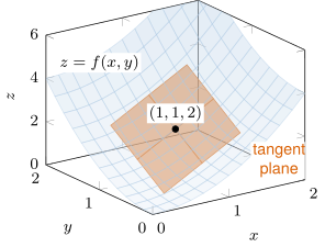
The figure shows the surface $z = f(x,y)$ for $f(x,y) = x^2 + y^2$ and, in orange, the plane tangent to the surface at the point $(1, 1, 2)$ . The point lies on the surface because $f(1,1) = 1^2 + 1^2 = 2$ . From $f_x = 2x$ and $f_y = 2y$ , the plane’s slope is $f_x(1,1) = 2(1) = 2$ in the $x$ -direction and $f_y(1,1) = 2(1) = 2$ in the $y$ -direction. The plane has the equation

z = 2 + 2(x - 1) + 2(y - 1).

Around $(1,1)$ , the plane and the surface nearly coincide. The plane is the graph of the linear approximation, defined next.

Definition 3 (Linear approximation in two inputs).

Let $f(x,y)$ be a smooth function around the point $(a,b)$ . The linear approximation of $f(x,y)$ when $(x,y) = (a,b)$ is given by

L(x,y) = f(a,b) + f_x(a,b)\cdot(x - a) + f_y(a,b)\cdot(y - b).

The function $k(x,y) = |x| + y$ has no linear approximation when $(x,y) = (0,0)$ , because it is not smooth around $(0,0)$ : section 2 of the Lesson 37 Notes shows that $k_x(0,0)$ does not exist. The definition requires a smooth function, and the formula for $L$ contains $k_x(0,0)$ .

The graph of $L(x,y)$ is a plane, the two-input counterpart of the tangent line of the single-variable linear approximation in section 1 of the Lesson 30 Notes. For inputs near $(a,b)$ , the linear approximation $L(x,y)$ estimates $f(x,y)$ .

Finding a linear approximation.

Compute the first partial derivatives $f_x$ and $f_y$ .
Evaluate $f$ , $f_x$ , and $f_y$ at $(a,b)$ .
Substitute $f(a,b)$ , $f_x(a,b)$ , and $f_y(a,b)$ into $L(x,y)$ and leave $x$ and $y$ as variables.

Example 9

Find the linear approximation of $f(x,y)$ when $(x,y) = (1,2)$ , and use it to estimate $f(1.1, 1.9)$ :

f(x,y) = xy + e^{xy}.

ShowHide solution

By the definition of the linear approximation, the linear approximation at $(a,b) = (1,2)$ is

L(x,y) = f(1,2) + f_x(1,2)\cdot(x - 1) + f_y(1,2)\cdot(y - 2).

To write the approximation, find the output $f(1,2)$ and the two slopes $f_x(1,2)$ and $f_y(1,2)$ .

Compute the first partial derivatives. The chain rule gives $\frac{\partial}{\partial x}\bigl[e^{xy}\bigr] = ye^{xy}$ and $\frac{\partial}{\partial y}\bigl[e^{xy}\bigr] = xe^{xy}$ :

f_x = \frac{\partial}{\partial x}\bigl[xy + e^{xy}\bigr] = y + ye^{xy}, \qquad f_y = \frac{\partial}{\partial y}\bigl[xy + e^{xy}\bigr] = x + xe^{xy}.

Evaluate $f$ , $f_x$ , and $f_y$ at $(1,2)$ :

\begin{align*} f(1,2) &= (1)(2) + e^{(1)(2)} = 2 + e^2,\\ f_x(1,2) &= 2 + 2e^{(1)(2)} = 2 + 2e^2,\\ f_y(1,2) &= 1 + 1 \cdot e^{(1)(2)} = 1 + e^2. \end{align*}

Substitute the three values into the linear approximation:

L(x,y) = (2 + e^2) + (2 + 2e^2)(x - 1) + (1 + e^2)(y - 2).

Evaluate $L$ at $(1.1, 1.9)$ , keeping $e^2$ exact until the last step. Used calculator.

\begin{align*} L(1.1, 1.9) &= (2 + e^2) + (2 + 2e^2)(1.1 - 1) + (1 + e^2)(1.9 - 2)\\ &= (2 + e^2) + (0.2 + 0.2e^2) + (-0.1 - 0.1e^2)\\ &= 2.1 + 1.1e^2 \approx 10.228. \end{align*}

As a check, the actual value is

f(1.1, 1.9) = (1.1)(1.9) + e^{(1.1)(1.9)} = 2.09 + e^{2.09} \approx 10.175,

below the estimate 10.228 by about 0.053.

Example 10

Use R to build the linear approximation of $f(x,y) = xy + e^{xy}$ when $(x,y) = (1,2)$ , and compute the estimate of $f(1.1, 1.9)$ .

ShowHide solution

Define $f$ , compute $f_x$ and $f_y$ with D(), and evaluate all three at $(1,2)$ . Used R.

f = makeFun(x*y + exp(x*y) ~ x & y)
dfx = D(f(x,y) ~ x)
dfy = D(f(x,y) ~ y)
f(x = 1, y = 2)
[1] 9.389056
dfx(x = 1, y = 2)
[1] 16.77811
dfy(x = 1, y = 2)
[1] 8.389056

As a check by hand, $f_x = y + ye^{xy}$ and $f_y = x + xe^{xy}$ give $f(1,2) = 2 + e^2$ , $f_x(1,2) = 2 + 2e^2$ , and $f_y(1,2) = 1 + e^2$ , which match R with $e^2 \approx 7.389056$ . The linear approximation is

L(x,y) \approx 9.389 + 16.778(x - 1) + 8.389(y - 2).

Build $L$ from the unrounded R values and evaluate it at $(1.1, 1.9)$ :

L = makeFun(f(1, 2) + dfx(1, 2)*(x - 1) +
dfy(1, 2)*(y - 2) ~ x & y)
L(x = 1.1, y = 1.9)
[1] 10.22796

The estimate is $f(1.1, 1.9) \approx L(1.1, 1.9) \approx 10.228$ .

Example 11

A linear approximation of a function $f(x,y)$ is

L(x,y) = 5 - 2(x - 3) + 4(y + 1).

Determine the point $(a,b)$ at which $L$ approximates $f$ , the value of $f$ at that point, and whether $f$ increases or decreases in each input near that point.

ShowHide solution

Rewrite $y + 1$ as $y - (-1)$ and match the terms to the linear approximation formula:

L(x,y) = 5 + (-2)\cdot(x - 3) + 4\cdot\bigl(y - (-1)\bigr) = f(a,b) + f_x(a,b)\cdot(x - a) + f_y(a,b)\cdot(y - b).

The match gives $a = 3$ and $b = -1$ . The linear approximation is taken at $(3, -1)$ , where $f(3,-1) = 5$ . Near that point, $f$ decreases in $x$ because $f_x(3,-1) = -2$ is negative. It increases in $y$ because $f_y(3,-1) = 4$ is positive.

Example 12

A cylinder with radius $r$ centimeters and height $h$ centimeters has volume

\text{Vol}(r,h) = \pi r^2 h

cubic centimeters. Find the linear approximation of Vol when $(r,h) = (2,5)$ , and use it to estimate the volume when the radius is 2.1 centimeters and the height is 4.9 centimeters.

ShowHide solution

To write the linear approximation, find $\text{Vol}(2,5)$ , $\text{Vol}_r(2,5)$ , and $\text{Vol}_h(2,5)$ . Compute the first partial derivatives. With respect to $r$ , the factor $\pi h$ is a constant multiple. With respect to $h$ , the factor $\pi r^2$ is a constant multiple:

\text{Vol}_r = \frac{\partial}{\partial r}\bigl[\pi r^2 h\bigr] = 2\pi rh, \qquad \text{Vol}_h = \frac{\partial}{\partial h}\bigl[\pi r^2 h\bigr] = \pi r^2.

Evaluate all three at $(2,5)$ :

\begin{align*} \text{Vol}(2,5) &= \pi(2)^2(5) = 20\pi,\\ \text{Vol}_r(2,5) &= 2\pi(2)(5) = 20\pi,\\ \text{Vol}_h(2,5) &= \pi(2)^2 = 4\pi. \end{align*}

Substitute the three values into the linear approximation:

L(r,h) = 20\pi + 20\pi(r - 2) + 4\pi(h - 5).

Evaluate $L$ at $(2.1, 4.9)$ . Used calculator.

\begin{align*} L(2.1, 4.9) &= 20\pi + 20\pi(2.1 - 2) + 4\pi(4.9 - 5)\\ &= 20\pi + 2\pi - 0.4\pi = 21.6\pi \approx 67.858. \end{align*}

The estimated volume is about 67.858 cubic centimeters. As a check, the actual volume is

\text{Vol}(2.1, 4.9) = \pi(2.1)^2(4.9) = 21.609\pi \approx 67.887

cubic centimeters. The actual volume is above the estimate $21.6\pi$ by $0.009\pi \approx 0.028$ cubic centimeters.

Lesson map