Lesson 26: Limits and the Derivative

Objectives

Understand when a limit exists; understand and write limit notation.
Visually and numerically estimate a limit, or justify why it does not exist.
Determine if a function is continuous at an input using the limit definition of continuity; understand that certain combinations of modeling functions are continuous on their domains.
Understand and apply the limit definition of the derivative to estimate a derivative at a given input.

1. Limits

Objective. Understand when a limit exists; understand and write limit notation.

Definition 1 (Limit).

The limit of a function $f(x)$ as the variable $x$ approaches a number $a$ is the number that the outputs of $f(x)$ approach as the inputs $x$ get close (but not necessarily equal) to $a$ from both the left and the right, and is denoted by $\displaystyle\lim_{x\to a} f(x)$ . If $f(x)$ does not approach a unique number, then $\displaystyle\lim_{x\to a} f(x)$ does not exist. The notation $\displaystyle\lim_{x\to 2} f(x) = 15$ reads “the limit of $f(x)$ as $x$ approaches 2 is 15.”

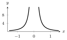
The function $f(x) = 1/x^2$ has no limit as $x$ approaches 0. Its outputs $f(\pm 0.1) = 100$ , $f(\pm 0.01) = 10{,}000$ , and $f(\pm 0.001) = 1{,}000{,}000$ rise without bound, and the definition requires the outputs to approach a unique number.

Dots on a graph. A filled dot at $x = a$ marks the value $f(a)$ , and an open dot at $x = a$ marks a point missing from the graph.

Limit and function value. The limit does not depend on $f(a)$ . Each graph below shows a function whose outputs approach 3 as $x$ approaches 2. In all three, $\displaystyle\lim_{x\to 2} f(x) = 3$ .

Value equal to the limit

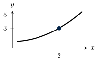
The filled dot on the curve gives $f(2) = 3$ , the same number as the limit.

Value different from the limit

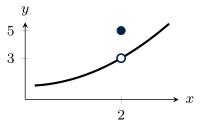
The filled dot above the curve gives $f(2) = 5$ , and the limit is still 3.

Undefined value

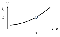
The open dot marks $f(2)$ as undefined, and the limit is still 3.

The left-hand limit of a function $f(x)$ as $x$ approaches $a$ is the number that the outputs of $f(x)$ approach as the inputs $x$ get close to $a$ through values less than $a$ , and is denoted by $\displaystyle\lim_{x\to a^-} f(x)$ .

The right-hand limit of a function $f(x)$ as $x$ approaches $a$ is the number that the outputs of $f(x)$ approach as the inputs $x$ get close to $a$ through values greater than $a$ , and is denoted by $\displaystyle\lim_{x\to a^+} f(x)$ .

Limit notation. Each notation reads as follows.

Notation	Reading
$\displaystyle\lim_{x\to a} f(x)$	the limit of $f(x)$ as $x$ approaches $a$
$\displaystyle\lim_{x\to a^-} f(x)$	the left-hand limit of $f(x)$ as $x$ approaches $a$
$\displaystyle\lim_{x\to a^+} f(x)$	the right-hand limit of $f(x)$ as $x$ approaches $a$

Theorem 2 (Existence of a limit).

The limit $\displaystyle\lim_{x\to a} f(x)$ exists exactly when the left-hand limit and the right-hand limit both exist and are equal.

Example 1

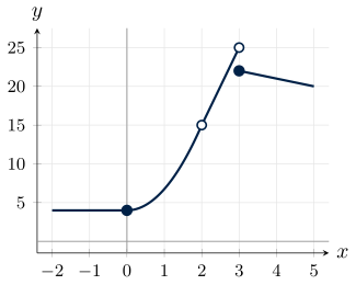
Evaluate each limit using the graph of $f(x)$ , or explain why the limit does not exist:

\text{(a)}\ \lim_{x\to 0} f(x), \qquad \text{(b)}\ \lim_{x\to 2} f(x), \qquad \text{(c)}\ \lim_{x\to 3} f(x).

ShowHide solution

By the definition of a limit, $\displaystyle\lim_{x\to 0} f(x)$ equals 4, because the outputs approach 4 as the inputs approach 0 from both the left and the right.
The limit $\displaystyle\lim_{x\to 2} f(x)$ equals 15, because the outputs approach 15 as the inputs approach 2 from both sides. The value $f(2)$ is undefined, because the graph has an open dot at $(2, 15)$ .
The limit $\displaystyle\lim_{x\to 3} f(x)$ does not exist, because $\displaystyle\lim_{x\to 3^-} f(x) = 25$ , at the open dot, and $\displaystyle\lim_{x\to 3^+} f(x) = 22$ , at the filled dot, are different numbers.

Example 2

A parking garage charges $C(t)$ dollars to park for $t$ hours. As $t$ approaches 2 through times less than 2 hours, the charge approaches 10 dollars. As $t$ approaches 2 through times greater than 2 hours, the charge approaches 15 dollars. Write both statements in limit notation, and determine whether $\displaystyle\lim_{t\to 2} C(t)$ exists.

ShowHide solution

By the definitions of the left-hand and right-hand limits, the two statements are

\lim_{t\to 2^-} C(t) = 10, \qquad \lim_{t\to 2^+} C(t) = 15.

The first reads “the left-hand limit of $C(t)$ as $t$ approaches 2 is 10.” By the existence of a limit theorem, $\displaystyle\lim_{t\to 2} C(t)$ does not exist, because the one-sided limits 10 and 15 are different numbers. Near 2 hours the charge approaches no single amount: it jumps by 5 dollars at 2 hours.

Lesson map

2. Estimating a Limit

Objective. Visually and numerically estimate a limit, or justify why it does not exist.

Limit from a graph.

Trace the graph toward $x = a$ from the left and read the height it approaches.
Trace the graph toward $x = a$ from the right and read the height it approaches.
Compare the two heights. Equal heights give the limit, and different heights mean the limit does not exist. A graph that rises or falls without bound on either side approaches no height, and the limit does not exist.

A limit that does not exist. The two graphs show the two ways a limit fails to exist in this course.

Different one-sided limits

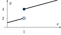
The limit as $x$ approaches 1 does not exist, because the outputs approach 2 from the left and 4 from the right.

Outputs without bound

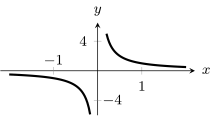
The limit as $x$ approaches 0 does not exist, because the outputs of $1/x$ rise without bound to the right of $x = 0$ and fall without bound to the left.

Example 3

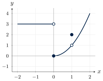
Evaluate each limit using the graph of $g(x)$ , or explain why the limit does not exist:

\text{(a)}\ \lim_{x\to -1} g(x), \qquad \text{(b)}\ \lim_{x\to 0} g(x), \qquad \text{(c)}\ \lim_{x\to 1} g(x).

ShowHide solution

The limit $\displaystyle\lim_{x\to -1} g(x)$ equals 3, because the graph is level at height 3 on both sides of $x = -1$ .
The limit $\displaystyle\lim_{x\to 0} g(x)$ does not exist, because $\displaystyle\lim_{x\to 0^-} g(x) = 3$ and $\displaystyle\lim_{x\to 0^+} g(x) = 0$ are different numbers.
The limit $\displaystyle\lim_{x\to 1} g(x)$ equals 1, because the outputs approach 1 as the inputs approach 1 from both sides. The filled dot gives $g(1) = 2$ .

Limit from a formula.

Choose inputs on each side of $a$ , such as $a - 0.1$ , $a - 0.01$ , and $a - 0.001$ on the left and $a + 0.001$ , $a + 0.01$ , and $a + 0.1$ on the right.
Evaluate the function at each input.
Compare the outputs. If the outputs on each side approach one number as the inputs get closer to $a$ , and the two sides agree, then that number is the estimate of the limit. If the two sides approach different numbers, or the outputs rise or fall without bound, then the limit does not exist.

Example 4

Numerically approximate the limit in R, with $x$ in radians:

\lim_{x\to 0} \frac{\sin(x)}{x}.

ShowHide solution

Define $g(x) = \dfrac{\sin(x)}{x}$ and evaluate it at inputs on each side of $x = 0$ and at $x = 0$ itself. Used R.

g = makeFun(sin(x)/x ~ x)
g(c(-0.1, -0.01, -0.001))
[1] 0.9983342 0.9999833 0.9999998
g(c(0.1, 0.01, 0.001))
[1] 0.9983342 0.9999833 0.9999998
g(0)
[1] NaN

R returns the three outputs in the order of the inputs inside c(). It returns NaN (not a number) for g(0), because $\frac{0}{0}$ is undefined. The outputs at $x = \pm 0.01$ and $x = \pm 0.001$ all round to 1.000, from both the left and the right. The numerical estimate of the limit is

\lim_{x\to 0} \frac{\sin(x)}{x} \approx 1.000.

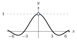
On the graph of $g$ , the curve approaches the dashed line at height 1 from both sides of $x = 0$ , and the open dot at $(0, 1)$ marks the point missing from the graph.

Example 5

Numerically approximate the limit in R, or justify why it does not exist:

\lim_{x\to 0} \frac{|x|}{x}.

ShowHide solution

Evaluate $s(x) = \dfrac{|x|}{x}$ on each side of $x = 0$ , as in Example 4. Used R.

s = makeFun(abs(x)/x ~ x)
s(c(-0.1, -0.01, -0.001))
[1] -1 -1 -1
s(c(0.1, 0.01, 0.001))
[1] 1 1 1

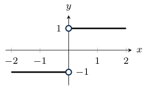
The limit does not exist, because the outputs approach $-1$ from the left and $1$ from the right. For every $x$ with $x < 0$ , $|x| = -x$ and $s(x) = -1$ . For every $x$ with $x > 0$ , $|x| = x$ and $s(x) = 1$ . The graph jumps from height $-1$ to height 1 at $x = 0$ .

Lesson map

3. Continuity

Objective. Determine if a function is continuous at an input using the limit definition of continuity; understand that certain combinations of modeling functions are continuous on their domains.

Definition 3 (Continuous).

A function $f(x)$ is continuous at $x = a$ if and only if

\lim_{x\to a} f(x) = f(a).

At an endpoint of the domain, such as $x = 0$ for $\sqrt{x}$ , the limit is the one-sided limit from inside the domain. A function $f(x)$ is continuous on its domain exactly when $f(x)$ is continuous at every input in its domain.

The function $q(x) = \dfrac{x^2 - 1}{x - 1}$ is not continuous at $x = 1$ . Its limit there exists, because for every $x$ with $x \neq 1$ ,

q(x) = \frac{(x - 1)(x + 1)}{x - 1} = x + 1.

As $x$ approaches 1, the outputs approach $1 + 1 = 2$ , and $\displaystyle\lim_{x\to 1} q(x) = 2$ . The value $q(1)$ is undefined, because substituting $x = 1$ gives $\frac{0}{0}$ . The definition requires the limit to equal $q(1)$ . Therefore $q(x)$ is not continuous at $x = 1$ .

Criterion 4 (Continuity).

A function $f(x)$ is continuous at $x = a$ exactly when all three conditions are true:

The value $f(a)$ is defined.
The limit $\displaystyle\lim_{x\to a} f(x)$ exists.
The limit $\displaystyle\lim_{x\to a} f(x)$ equals $f(a)$ .

As in the definition, at an endpoint of the domain the limits in the second and third conditions are one-sided.

A function is continuous on an interval when it is continuous at every input in the interval, and its graph over that interval can then be drawn without lifting the pen.

Failed conditions. Each function graphed below is not continuous at $x = a$ , and the first condition to fail is a different one in each.

Undefined value

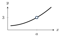
The first condition fails: the open dot marks $f(a)$ as undefined.

Limit nonexistent

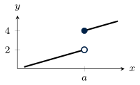
The second condition fails: the one-sided limits 2 and 4 differ.

Value different from the limit

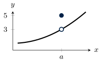
The third condition fails: the limit 3 differs from $f(a) = 5$ .

Example 6

Use the graph of $f(x)$ to determine whether $f(x)$ is continuous at $x = -2$ , at $x = 0$ , and at $x = 2$ .

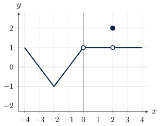
ShowHide solution

By the definition of continuous, $f(x)$ is continuous at $x = -2$ , because $\displaystyle\lim_{x\to -2} f(x) = -1$ equals $f(-2) = -1$ , the height of the corner at $(-2, -1)$ .
The function $f(x)$ is not continuous at $x = 0$ , because $f(0)$ is undefined: the graph has an open dot at $(0, 1)$ .
The function $f(x)$ is not continuous at $x = 2$ , because $\displaystyle\lim_{x\to 2} f(x) = 1$ and $f(2) = 2$ are not equal.

Theorem 5 (Continuous functions).

Linear, exponential, power, trigonometric, and sigmoidal functions are continuous on their domains.
A function built from the common modeling functions by sums, differences, products, quotients, and one function inside another is continuous on its domain.

The natural logarithm $\ln(x)$ is also continuous on its domain. An input that makes a denominator zero, or puts zero or a negative number into a logarithm, lies outside the domain of a combination of common modeling functions. So does an input that puts a negative number under an even root, such as a square root.

For a piecewise function whose pieces are continuous on their intervals, check the three conditions at each boundary between pieces.

If $f(x)$ is continuous at $x = a$ , then substituting $x = a$ into $f(x)$ gives $\displaystyle\lim_{x\to a} f(x)$ .

Example 7

Identify where each function is continuous:

a(x) = e^{\sin(3x)} + \frac{1}{\sqrt{x}}, \qquad b(x) = \frac{\cos(9x + 5)}{4x - 7}, \qquad c(x) = \begin{cases} 2 & x < 4 \\ 8x & x \geq 4 \end{cases}.

ShowHide solution

By the continuous functions theorem, $a(x)$ is continuous on $(0, \infty)$ , the inputs where both of its terms are continuous. The function $e^{\sin(3x)}$ , a sine inside an exponential, is continuous on all real numbers. The power function $\dfrac{1}{\sqrt{x}} = x^{-1/2}$ has domain $x > 0$ , because a square root of a negative number and division by zero are both undefined, and it is continuous on that domain.
By the continuous functions theorem, $b(x)$ is continuous on all real numbers except $x = \frac{7}{4}$ , because it is a quotient of continuous functions and $4x - 7 = 0$ at $x = \frac{7}{4}$ .
Because both pieces of $c(x)$ are linear, $x = 4$ is the only input to check. The one-sided limits at $x = 4$ are
$\lim_{x\to 4^-} c(x) = 2, \qquad \lim_{x\to 4^+} c(x) = 8(4) = 32.$
The limit $\displaystyle\lim_{x\to 4} c(x)$ does not exist, because the one-sided limits differ. Therefore $c(x)$ is continuous on all real numbers except $x = 4$ .

Example 8

Identify where the function is continuous:

d(x) = \begin{cases} x^2 & x < 0 \\ x & x \geq 0 \end{cases}.

ShowHide solution

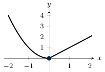
Because both pieces are continuous, $x = 0$ is the only input to check against the continuity criterion. The first condition is true, because $d(0) = 0$ from the piece for $x \geq 0$ . Substituting $x = 0$ into each continuous piece gives the one-sided limits $\displaystyle\lim_{x\to 0^-} x^2 = 0$ and $\displaystyle\lim_{x\to 0^+} x = 0$ . By the existence of a limit theorem, $\displaystyle\lim_{x\to 0} d(x) = 0$ , and this limit equals $d(0)$ . The second and third conditions are true. Therefore $d(x)$ is continuous on all real numbers. On the graph, the parabola $y = x^2$ from the left and the line $y = x$ from the right meet at $(0, d(0)) = (0, 0)$ , and the graph can be drawn without lifting the pen.

Lesson map

4. Limit Definition of the Derivative

Objective. Understand and apply the limit definition of the derivative to estimate a derivative at a given input.

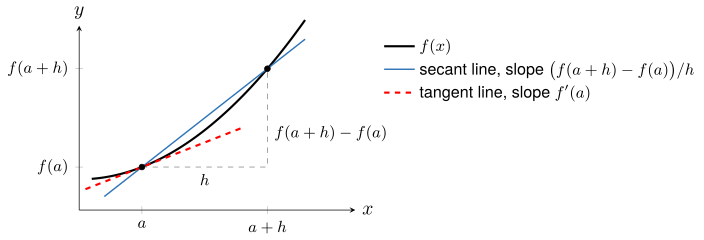
The secant line through $(a, f(a))$ and $(a + h, f(a + h))$ has slope $\bigl(f(a + h) - f(a)\bigr)/h$ , the average rate of change of $f(x)$ over the interval between $a$ and $a + h$ (Lesson 25 Notes, section 1). As $h$ approaches 0, the point $(a + h, f(a + h))$ slides along the graph toward $(a, f(a))$ , and, when $f'(a)$ exists, the secant line approaches the tangent line. A positive $h$ gives an interval to the right of $a$ , and a negative $h$ gives an interval to the left of $a$ .

Definition 6 (Limit definition of the derivative).

By the limit definition of the derivative, the derivative of a function $f(x)$ for input $x = a$ is

f'(a) = \lim_{h\to 0} \frac{f(a + h) - f(a)}{h}.

The derivative $f'(a)$ is the instantaneous rate of change of $f(x)$ when $x = a$ (Lesson 25 Notes, section 3). It exists only when, as $h$ approaches 0, the average rates of change from both sides of $a$ approach the same number.

The function $c(x)$ of Example 7, equal to 2 for $x < 4$ and to $8x$ for $x \geq 4$ , has no derivative when $x = 4$ . The piece $8x$ gives its value there, $c(4) = 32$ . For every $h$ with $h < 0$ , the average rate of change in the definition is

\frac{c(4 + h) - c(4)}{h} = \frac{2 - 32}{h} = \frac{-30}{h},

which rises without bound as $h$ approaches 0 from the left. The definition requires the average rate of change to approach a number.

Estimating a derivative.

Substitute the function and the input $a$ into the definition.
Compute the average rate of change for values of $h$ on both sides of 0 that shrink by a factor of 10, such as $h = \pm 0.001$ , $\pm 0.0001$ , and $\pm 0.00001$ .
Apply the stopping test from the Lesson 25 Notes, section 2: stop at a step where, to three decimals, the rates for $+h$ and $-h$ agree with each other and with the rates on the step before.
Report the number the average rates of change approach from both sides, with units. If the two sides approach different numbers, or the rates rise or fall without bound, then the derivative does not exist.

Example 9

Write the limit definition of $f'(2)$ and use it to estimate $f'(2)$ in R:

f(x) = 3x^2 - 2x.

ShowHide solution

By the limit definition of the derivative,

f'(a) = \lim_{h\to 0} \frac{f(a + h) - f(a)}{h}.

Calculate $f(2)$ , the value subtracted in the numerator:

f(2) = 3(2)^2 - 2(2) = 12 - 4 = 8.

Substitute $f(x)$ , $a = 2$ , and $f(2) = 8$ into the limit definition of the derivative:

f'(2) = \lim_{h\to 0} \frac{3(2 + h)^2 - 2(2 + h) - 8}{h}.

Compute the average rate of change in the definition for $h = \pm 0.001$ , $\pm 0.0001$ , and $\pm 0.00001$ . Used R.

f = makeFun(3*x^2 - 2*x ~ x)
h = c(0.001, 0.0001, 0.00001, -0.001, -0.0001, -0.00001)
(f(2 + h) - f(2))/h
[1] 10.00300 10.00030 10.00003  9.99700  9.99970  9.99997

The line h = c(...) stores the six values of $h$ . The line (f(2 + h) - f(2))/h computes the average rate of change in the definition for each one, and R prints the six quotients in the same order, the three positive values of $h$ first. At $h = \pm 0.001$ the average rates of change round to 10.003 and 9.997. At $h = \pm 0.0001$ and at $h = \pm 0.00001$ all four round to 10.000. The stopping test is met:

f'(2) \approx 10.000.

Example 10

The median home price $P$ in the United States, in thousands of dollars, in year $Y$ from 2001 to 2010 is modeled by

P(Y) = 0.17(Y - 2001)^4 - 3.2(Y - 2001)^3 + 16.7(Y - 2001)^2 - 10.9(Y - 2001) + 177.7.

Estimate $P'(2005)$ in R using the limit definition of the derivative, and explain what the value means.

ShowHide solution

The limit definition of the derivative when $Y = 2005$ is

P'(2005) = \lim_{h\to 0} \frac{P(2005 + h) - P(2005)}{h}.

Estimate the limit as in Example 9, with $h = \pm 0.0001$ , $\pm 0.00001$ , and $\pm 0.000001$ . Used R.

P = makeFun(0.17*(Y - 2001)^4 - 3.2*(Y - 2001)^3 +
16.7*(Y - 2001)^2 - 10.9*(Y - 2001) + 177.7 ~ Y)
h = c(0.0001, 0.00001, 0.000001, -0.0001, -0.00001, -0.000001)
(P(2005 + h) - P(2005))/h
[1] 12.61946 12.61995 12.62000 12.62054 12.62005 12.62001

At $h = \pm 0.0001$ the average rates of change round to 12.619 and 12.621. At $h = \pm 0.00001$ and at $h = \pm 0.000001$ all four round to 12.620. The stopping test is met:

P'(2005) \approx 12.620.

The units are thousand dollars per year, and the dimension is $[P]/[Y] = BT^{-1}$ . Based on the model, the median home price was increasing at about $12,620 per year in 2005.

Example 11

Use the limit definition of the derivative, with average rates of change computed in R, to show that $f'(0)$ does not exist:

f(x) = |x|.

ShowHide solution

Substituting $f(x) = |x|$ and $a = 0$ into the limit definition of the derivative gives

f'(0) = \lim_{h\to 0} \frac{|0 + h| - |0|}{h} = \lim_{h\to 0} \frac{|h|}{h},

the limit of Example 5 with $h$ in place of $x$ . Compute the average rate of change $\dfrac{|h|}{h}$ for $h = \pm 0.1$ , $\pm 0.01$ , and $\pm 0.001$ . Used R.

f = makeFun(abs(x) ~ x)
h = c(0.1, 0.01, 0.001, -0.1, -0.01, -0.001)
(f(0 + h) - f(0))/h
[1]  1  1  1 -1 -1 -1

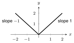
The average rates of change equal 1 for positive $h$ , because $|h| = h$ there, and $-1$ for negative $h$ , because $|h| = -h$ there. Because they approach different numbers from the two sides, $f'(0)$ does not exist. The graph of $|x|$ shows the same fact as a corner at $(0, 0)$ , where the slope is $-1$ on the left and 1 on the right.

Lesson map