Lesson 37: Partial Derivatives I

Objectives

Given a tabular function or contour plot, approximate the rate of change at a point with respect to each input variable.
Describe the partial derivative as the instantaneous rate of change with respect to a single input.
Compute partial derivatives by hand using derivative rules.
Write and understand Leibniz (“fraction with curly d”) and subscript notation for partials.

1. Rates of Change from Tables and Contour Plots

Objective. Given a tabular function or contour plot, approximate the rate of change at a point with respect to each input variable.

With one input held constant, a row or column of a table is a function of the other input. Along a horizontal or vertical line across a contour plot, the output is also a function of one input.

Definition 1 (Average rate of change with respect to an input).

For a multivariable function $f(x,y)$ , the average rate of change with respect to $x$ of $f(x,y)$ over an $x$ -interval $[a, c]$ when $y = b$ is given by

\frac{f(c,b) - f(a,b)}{c - a}.

For a multivariable function $f(x,y)$ , the average rate of change with respect to $y$ of $f(x,y)$ over a $y$ -interval $[b, d]$ when $x = a$ is given by

\frac{f(a,d) - f(a,b)}{d - b}.

The two points $(1, 0.5)$ and $(1.1, 1)$ give no average rate of change with respect to $x$ , because $y$ changes from 0.5 to 1 along with $x$ . The definition requires the same value $y = b$ at both points.

To approximate the rate of change at a point, choose the input interval by these rules:

Make the interval as small as the available information allows.
Make the interval contain the input where the rate is approximated.

Side of the interval on a table. On a table, two intervals of the smallest width contain an input away from the table’s edges: one ending at it and one starting at it. The two intervals can give different estimates, as in Example 2. Every table example here uses the interval that starts at the input and runs toward larger inputs. Because the temperatures on the wind chill chart decrease from left to right, the interval that starts at $15^\circ$ F runs left to $20^\circ$ F. When a problem gives the interval, use the interval given.

Units. A rate of change carries the output units per unit of the chosen input. The rate of change of wind chill in $^\circ$ F with respect to wind speed in mph is in $^\circ$ F per mph.

The National Weather Service wind chill chart gives the wind chill $WC(T, V)$ in $^\circ$ F for air temperature $T$ in $^\circ$ F and wind speed $V$ in mph. The table reproduces part of the chart.

	Temperature $T$ ( $^\circ$ F)
$V$ (mph)	20	15	10	5	0	$-5$	$-10$
5	13	7	1	$-5$	$-11$	$-16$	$-22$
10	9	3	$-4$	$-10$	$-16$	$-22$	$-28$
15	6	0	$-7$	$-13$	$-19$	$-26$	$-32$
20	4	$-2$	$-9$	$-15$	$-22$	$-29$	$-35$
25	3	$-4$	$-11$	$-17$	$-24$	$-31$	$-37$
30	1	$-5$	$-12$	$-19$	$-26$	$-33$	$-39$
35	0	$-7$	$-14$	$-21$	$-27$	$-34$	$-41$

Example 1

At an air temperature of $5^\circ$ F, approximate the rate of change of wind chill with respect to wind speed between 10 and 15 mph.

ShowHide solution

By the definition of average rate of change with respect to an input, hold $T$ at 5. The average rate of change with respect to $V$ over $[10, 15]$ is

\frac{WC(5, 15) - WC(5, 10)}{15 - 10}.

Read $WC(5, 15) = -13$ and $WC(5, 10) = -10$ from the $5^\circ$ F column and substitute them into the formula:

\frac{WC(5, 15) - WC(5, 10)}{15 - 10} = \frac{-13 - (-10)}{5} = \frac{-3}{5} = -0.6.

At $5^\circ$ F, the wind chill decreases about $0.6^\circ$ F per mph of wind speed between 10 and 15 mph.

Example 2

Approximate the rate of change of wind chill with respect to air temperature when the temperature is $-5^\circ$ F and the wind speed is 30 mph.

ShowHide solution

Hold $V$ at 30. The interval starts at $-5$ and runs up to 0, the next temperature on the chart. Read both wind chills from the 30 mph row and substitute them as in Example 1:

\frac{WC(0, 30) - WC(-5, 30)}{0 - (-5)} = \frac{-26 - (-33)}{5} = \frac{7}{5} = 1.4.

At $-5^\circ$ F and 30 mph, the wind chill increases about $1.4^\circ$ F per $^\circ$ F of air temperature. The interval $[-10, -5]$ on the other side gives $\bigl(-33 - (-39)\bigr)/5 = 1.2$ .

Contour plots. When no interval is given, estimate the rate of change at a point between two contours by these steps:

Draw the line through the point along which only the chosen input changes: horizontal for $x$ , vertical for $y$ . Find the two crossing points, where that line crosses the nearest contour on each side of the point.
Read the labels of the two contours as in section 2 of the Lesson 36 Notes. Take the change in output as the label at the crossing point with the larger input minus the label at the crossing point with the smaller input.
Take the change in input as the larger input minus the smaller input at the two crossing points, and divide the change in output by it.

The sign of the rate comes from the order of the contour labels along the line. In each graph, $f(x,y)$ is the elevation in meters at the map point $(x,y)$ , with $x$ increasing to the east, and the arrow runs east from the point.

Positive rate

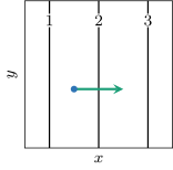
The rate with respect to $x$ is positive, because the labels increase toward the east. The ground rises to the east.

Negative rate

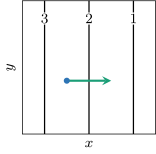
The rate with respect to $x$ is negative, because the labels decrease toward the east. The ground falls to the east.

Zero rate

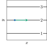
The rate with respect to $x$ is 0, because the arrow runs along the level 2 contour. The elevation stays at 2 meters to the east.

Values between contours. A point between two contours with different labels has a value between their labels. Estimate the value of $f$ at the point as in Example 5:

Draw the horizontal or vertical line through the point, and find where it crosses the two contours.
Find the fraction: the distance from the lower-labeled crossing to the point, divided by the distance from the lower-labeled crossing to the higher-labeled crossing.
Go that same fraction of the way from the lower label to the higher label.

A point inside the innermost closed contour has a value beyond that contour’s label: above it when the labels increase toward the point, below it when they decrease.

When a problem gives the interval, estimate $f$ at each endpoint from the contours and use the average rate of change formula.

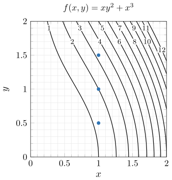
Example 3

Use the contour plot of

f(x,y) = xy^2 + x^3

above to approximate the rate of change of $f$ with respect to $x$ at $(1, 0.5)$ .

ShowHide solution

The point $(1, 0.5)$ lies between the contours labeled 1 and 2.

Along the line $y = 0.5$ , those contours cross at $x \approx 0.917$ and $x \approx 1.194$ , the ends of the green segment in the enlarged view. Divide the change in output between the two crossing points by the change in input:

\frac{2 - 1}{1.194 - 0.917} = \frac{1}{0.277} \approx 3.6.

At $(1, 0.5)$ , the function $f$ increases about 3.6 per unit of $x$ .

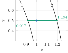
Example 4

Use the contour plot of

f(x,y) = xy^2 + x^3

above to approximate the rate of change of $f$ with respect to $y$ at $(1, 1.5)$ .

ShowHide solution

The point $(1, 1.5)$ lies between the contours labeled 3 and 4.

Along the line $x = 1$ , those contours cross at $y \approx 1.414$ and $y \approx 1.732$ , the ends of the purple segment in the enlarged view. Divide as in Example 3:

\frac{4 - 3}{1.732 - 1.414} = \frac{1}{0.318} \approx 3.1.

At $(1, 1.5)$ , the function $f$ increases about 3.1 per unit of $y$ .

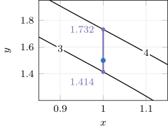
Example 5

Use the contour plot of

f(x,y) = xy^2 + x^3

above to approximate the average rate of change of $f$ with respect to $y$ over the interval $[1, 1.5]$ when $x = 1$ .

ShowHide solution

Estimate $f(1, 1)$ and $f(1, 1.5)$ from the contours, then substitute both into the formula for the average rate of change with respect to $y$ .

The point $(1, 1)$ lies on the contour labeled 2, which gives $f(1, 1) \approx 2$ . The point $(1, 1.5)$ lies between the contours labeled 3 and 4, which cross the line $x = 1$ at $y \approx 1.414$ and $y \approx 1.732$ , read in the enlarged view of Example 4. Find the fraction of the distance from the level 3 crossing to the level 4 crossing that lies between the level 3 crossing and the point:

\frac{1.5 - 1.414}{1.732 - 1.414} = \frac{0.086}{0.318} \approx 0.27.

Go the same fraction of the way from 3 to 4:

f(1, 1.5) \approx 3 + 0.27(4 - 3) = 3.27.

Substitute both values into the formula:

\frac{f(1, 1.5) - f(1, 1)}{1.5 - 1} \approx \frac{3.27 - 2}{0.5} = \frac{1.27}{0.5} \approx 2.5.

Over $1 \le y \le 1.5$ with $x = 1$ , the function $f$ increases about 2.5 per unit of $y$ .

Lesson map

2. The Partial Derivative

Objective. Describe the partial derivative as the instantaneous rate of change with respect to a single input.

A partial derivative is an instantaneous rate of change with respect to a single input. Section 2 of the Lesson 25 Notes defines the instantaneous rate of change.

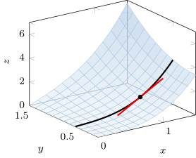
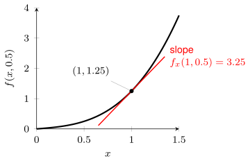
The left graph is the surface of $f(x,y) = xy^2 + x^3$ . Fixing $y = 0.5$ cuts the surface along the black curve, the graph of the one-input function $f(x, 0.5) = 0.25x + x^3$ , drawn alone on the right. The red line is tangent to that curve where $x = 1$ , at the height $f(1, 0.5) = 1.25$ . Its slope 3.25 is the partial derivative $f_x(1, 0.5)$ , defined next. This value is estimated in Example 6 and computed in Example 8.

Definition 2 (Partial derivative).

The partial derivative of $f(x,y)$ with respect to $x$ when $(x,y) = (a,b)$ is the number approached by the average rates of change with respect to $x$ of $f(x,y)$ when these rates are computed over smaller and smaller $x$ -intervals containing $x = a$ while $y = b$ is held constant. This first partial is denoted by $f_x(a,b)$ .

The partial derivative of $f(x,y)$ with respect to $y$ when $(x,y) = (a,b)$ is the number approached by the average rates of change with respect to $y$ of $f(x,y)$ when these rates are computed over smaller and smaller $y$ -intervals containing $y = b$ while $x = a$ is held constant. This first partial is denoted by $f_y(a,b)$ .

Geometrically, the partial derivative $f_x(a,b)$ is the slope of the line tangent to the surface of $f$ at the point $(a, b, f(a,b))$ in the $x$ -direction. The partial derivative $f_y(a,b)$ is the slope of the line tangent to the surface of $f$ at the point $(a, b, f(a,b))$ in the $y$ -direction.

The function $k(x,y) = |x| + y$ has no partial derivative with respect to $x$ when $(x,y) = (0,0)$ . With $y = 0$ held constant, for every positive number $t$ , its average rate of change with respect to $x$ over $[0, t]$ is $\bigl(|t| - 0\bigr)/t = 1$ , and over $[-t, 0]$ it is $\bigl(0 - |-t|\bigr)/t = -1$ . The average rates from the two sides stay apart, and the definition requires them to approach one number.

Example 6

For the function

f(x,y) = xy^2 + x^3

with $y = 0.5$ , compute the average rate of change of $f$ with respect to $x$ over each interval, and use the results to estimate $f_x(1, 0.5)$ :

[1, 1.1], \qquad [1, 1.01], \qquad [1, 1.001].

ShowHide solution

By the definition of the partial derivative, $f_x(1, 0.5)$ is the number that the average rates of change with respect to $x$ approach over smaller and smaller $x$ -intervals containing $x = 1$ , with $y = 0.5$ held constant. Every interval starts at $x = 1$ . Evaluate $f$ there once, with $y = 0.5$ :

f(1, 0.5) = 1(0.5)^2 + 1^3 = 0.25 + 1 = 1.25.

Over $[1, 1.1]$ , evaluate $f$ at the right endpoint and substitute both values into the formula for the average rate of change with respect to $x$ :

\begin{align*} f(1.1, 0.5) &= 1.1(0.5)^2 + 1.1^3 = 0.275 + 1.331 = 1.606,\\ \frac{f(1.1, 0.5) - f(1, 0.5)}{1.1 - 1} &= \frac{1.606 - 1.25}{0.1} = 3.56. \end{align*}

Over $[1, 1.01]$ , do the same:

\begin{align*} f(1.01, 0.5) &= 1.01(0.5)^2 + 1.01^3 = 0.2525 + 1.030301 = 1.282801,\\ \frac{f(1.01, 0.5) - f(1, 0.5)}{1.01 - 1} &= \frac{1.282801 - 1.25}{0.01} = 3.2801. \end{align*}

Over $[1, 1.001]$ , do the same:

\begin{align*} f(1.001, 0.5) &= 1.001(0.5)^2 + 1.001^3 = 0.25025 + 1.003003001 = 1.253253001,\\ \frac{f(1.001, 0.5) - f(1, 0.5)}{1.001 - 1} &= \frac{1.253253001 - 1.25}{0.001} = 3.253001. \end{align*}

The average rates of change approach 3.25, which gives the estimate $f_x(1, 0.5) \approx 3.25$ per unit of $x$ , with $y$ held at 0.5.

Example 7

A cylinder with radius $r$ centimeters and height $h$ centimeters has volume

\text{Vol}(r,h) = \pi r^2 h

cubic centimeters. With $h = 5$ , compute the average rate of change of Vol with respect to $r$ over each interval, and use the results to estimate $\text{Vol}_r(2, 5)$ , the partial derivative of Vol with respect to $r$ at $(2, 5)$ :

[2, 2.1], \qquad [2, 2.01], \qquad [2, 2.001].

Describe $\text{Vol}_r(2, 5)$ as an instantaneous rate of change, with its units.

ShowHide solution

Every interval starts at $r = 2$ . Evaluate Vol there once, with $h = 5$ :

\text{Vol}(2, 5) = \pi(2)^2(5) = 20\pi.

Over $[2, 2.1]$ , evaluate Vol at the right endpoint and substitute both values:

\begin{align*} \text{Vol}(2.1, 5) &= \pi(2.1)^2(5) = 22.05\pi,\\ \frac{\text{Vol}(2.1, 5) - \text{Vol}(2, 5)}{2.1 - 2} &= \frac{22.05\pi - 20\pi}{0.1} = 20.5\pi \approx 64.403. \end{align*}

Over $[2, 2.01]$ , do the same:

\begin{align*} \text{Vol}(2.01, 5) &= \pi(2.01)^2(5) = 20.2005\pi,\\ \frac{\text{Vol}(2.01, 5) - \text{Vol}(2, 5)}{2.01 - 2} &= \frac{20.2005\pi - 20\pi}{0.01} = 20.05\pi \approx 62.989. \end{align*}

Over $[2, 2.001]$ , do the same:

\begin{align*} \text{Vol}(2.001, 5) &= \pi(2.001)^2(5) = 20.020005\pi,\\ \frac{\text{Vol}(2.001, 5) - \text{Vol}(2, 5)}{2.001 - 2} &= \frac{20.020005\pi - 20\pi}{0.001} = 20.005\pi \approx 62.848. \end{align*}

The multiples of $\pi$ approach $20\pi$ , which gives the estimate

\text{Vol}_r(2, 5) \approx 20\pi \approx 62.832.

The partial derivative $\text{Vol}_r(2, 5)$ is the instantaneous rate of change of volume with respect to radius. When the radius is 2 centimeters and the height is held at 5 centimeters, the volume is increasing at about 62.832 cubic centimeters per centimeter of radius.

Lesson map

3. Computing Partial Derivatives

Objective. Compute partial derivatives by hand using derivative rules.

The derivative rules for one input apply to each partial derivative. Computed at every point $(x,y)$ instead of one point $(a,b)$ , the partial derivatives are functions $f_x(x,y)$ and $f_y(x,y)$ .

Find $f_x(x,y)$ by differentiating $f(x,y)$ with respect to $x$ while treating $y$ as a constant.
Find $f_y(x,y)$ by differentiating $f(x,y)$ with respect to $y$ while treating $x$ as a constant.

The symbol $\dfrac{\partial }{\partial x}\bigl[\ \bigr]$ stands for the partial derivative with respect to $x$ of the expression in the brackets. The notation is set out in full in section 4.

Constants. With respect to $x$ , a term with no $x$ in it differentiates to 0, and a factor with no $x$ in it is a constant multiple. In the term $xy^2$ , for example, the factor $y^2$ is a constant multiple. The constant multiple rule then applies in place of the product rule: $\dfrac{\partial }{\partial x}\bigl[xy^2\bigr] = y^2$ . The term $y^2$ alone is a constant: $\dfrac{\partial }{\partial x}\bigl[y^2\bigr] = 0$ .

Example 8

Compute both first partial derivatives of the function below, then evaluate $f_x(1, 0.5)$ and $f_y(1, 1.5)$ :

f(x,y) = xy^2 + x^3.

ShowHide solution

Find $f_x$ by differentiating with respect to $x$ while treating $y$ as a constant. The factor $y^2$ is then a constant multiple:

f_x(x,y) = \dfrac{\partial }{\partial x}\bigl[xy^2\bigr] + \dfrac{\partial }{\partial x}\bigl[x^3\bigr] = y^2(1) + 3x^2 = y^2 + 3x^2.

Substitute $x = 1$ and $y = 0.5$ into $f_x$ :

f_x(1, 0.5) = (0.5)^2 + 3(1)^2 = 0.25 + 3 = 3.25.

Find $f_y$ by differentiating with respect to $y$ while treating $x$ as a constant. The factor $x$ is then a constant multiple, and the term $x^3$ is a constant:

f_y(x,y) = \dfrac{\partial }{\partial y}\bigl[xy^2\bigr] + \dfrac{\partial }{\partial y}\bigl[x^3\bigr] = x(2y) + 0 = 2xy.

Substitute $x = 1$ and $y = 1.5$ into $f_y$ :

f_y(1, 1.5) = 2(1)(1.5) = 3.

The value $f_x(1, 0.5) = 3.25$ matches the estimate of Example 6 and is the slope of the red tangent line in the section 2 figure.

Example 9

Compute both first partial derivatives:

g(x,y) = x^2y - \ln(y).

ShowHide solution

With respect to $x$ , the factor $y$ is a constant multiple and the term $\ln(y)$ is a constant:

g_x(x,y) = y \cdot 2x - 0 = 2xy.

With respect to $y$ , the factor $x^2$ is a constant multiple:

g_y(x,y) = x^2 \cdot 1 - \frac{1}{y} = x^2 - \frac{1}{y}.

Example 10

Compute both first partial derivatives:

h(x,y) = 7e^{x^2 + 9y}.

ShowHide solution

By the chain rule, the partial derivative of $7e^{x^2 + 9y}$ is $7e^{x^2 + 9y}$ multiplied by the partial derivative of its exponent. With respect to $x$ , the exponent $x^2 + 9y$ has partial derivative $2x$ :

h_x(x,y) = 7e^{x^2 + 9y} \cdot 2x = 14x\,e^{x^2 + 9y}.

With respect to $y$ , the exponent has partial derivative 9:

h_y(x,y) = 7e^{x^2 + 9y} \cdot 9 = 63e^{x^2 + 9y}.

Example 11

Compute both first partial derivatives:

a(x,y) = e^{4x}\cos(xy).

ShowHide solution

With respect to $x$ , both factors contain $x$ and the product rule applies. By the chain rule, the partial derivative of $\cos(xy)$ with respect to $x$ is $-\sin(xy)$ multiplied by the partial derivative of $xy$ with respect to $x$ , which is $y$ :

a_x(x,y) = \cos(xy)\cdot 4e^{4x} + e^{4x}\cdot\bigl(-y\sin(xy)\bigr) = 4e^{4x}\cos(xy) - ye^{4x}\sin(xy).

With respect to $y$ , the factor $e^{4x}$ is a constant multiple. By the chain rule, the partial derivative of $\cos(xy)$ with respect to $y$ is $-\sin(xy)$ multiplied by the partial derivative of $xy$ with respect to $y$ , which is $x$ :

a_y(x,y) = e^{4x}\cdot\bigl(-x\sin(xy)\bigr) = -xe^{4x}\sin(xy).

Example 12

Compute both first partial derivatives:

q(x,y) = \frac{x + 1}{x + y^2}.

ShowHide solution

With respect to $x$ , the numerator and the denominator both contain $x$ and the quotient rule applies:

q_x(x,y) = \frac{(x + y^2)(1) - (x + 1)(1)}{(x + y^2)^2} = \frac{y^2 - 1}{(x + y^2)^2}.

With respect to $y$ , the numerator $x + 1$ is a constant multiple. Write $q$ as $(x + 1)(x + y^2)^{-1}$ and differentiate $(x + y^2)^{-1}$ by the chain rule:

q_y(x,y) = (x + 1)\cdot(-1)(x + y^2)^{-2}\cdot 2y = \frac{-2y(x + 1)}{(x + y^2)^2}.

Lesson map

4. Partial Derivative Notation

Objective. Write and understand Leibniz (“fraction with curly d”) and subscript notation for partials.

The symbol $\partial$ is the “curly d”, read “partial”. In both notations, the input that varies appears in the symbol.

Partial derivative	Subscript	Leibniz
With respect to $x$	$f_x(x,y)$	$\dfrac{\partial f}{\partial x}(x,y) = \dfrac{\partial }{\partial x}\bigl[f(x,y)\bigr]$
With respect to $y$	$f_y(x,y)$	$\dfrac{\partial f}{\partial y}(x,y) = \dfrac{\partial }{\partial y}\bigl[f(x,y)\bigr]$
With respect to $x$ at $(a,b)$	$f_x(a,b)$	$\dfrac{\partial f}{\partial x}(a,b)$

The symbol $f_x$ is read “ $f$ sub $x$ ”, and $\dfrac{\partial f}{\partial x}$ is read “partial $f$ partial $x$ ”. The symbol $f_x$ names a new function, the partial derivative of $f$ with respect to $x$ .

As in the textbook, each function in the examples is assumed to have partial derivatives at the points used in the examples.

A function has one first partial derivative for each input, defined in the same way for a third input $z$ : the function $g(x,y,z)$ has the three first partial derivatives $g_x$ , $g_y$ , and $g_z$ .

Example 13

Write the rate of change of wind chill with respect to wind speed at $-5^\circ$ F and 30 mph in subscript and Leibniz notation, and approximate it from the chart in section 1.

ShowHide solution

For the wind chill $WC(T, V)$ , the rate of change with respect to wind speed at $-5^\circ$ F and 30 mph is $WC_V(-5, 30)$ in subscript notation and $\dfrac{\partial WC}{\partial V}(-5, 30)$ in Leibniz notation. As in section 1, the wind speed interval starts at 30 mph and runs up to 35 mph, the next wind speed on the chart:

WC_V(-5, 30) = \dfrac{\partial WC}{\partial V}(-5, 30) \approx \frac{WC(-5, 35) - WC(-5, 30)}{35 - 30} = \frac{-34 - (-33)}{5} = -0.2.

Therefore, at $-5^\circ$ F and 30 mph the wind chill decreases about $0.2^\circ$ F per mph of wind speed.

Example 14

For the function

f(x,y) = xy^2 + x^3,

compute $\dfrac{\partial f}{\partial y}(2, -1)$ and write it in subscript notation.

ShowHide solution

Differentiate with respect to $y$ while treating $x$ as a constant:

f_y(x,y) = \dfrac{\partial }{\partial y}\bigl[xy^2\bigr] + \dfrac{\partial }{\partial y}\bigl[x^3\bigr] = x(2y) + 0 = 2xy.

Substitute $x = 2$ and $y = -1$ :

\dfrac{\partial f}{\partial y}(2, -1) = f_y(2, -1) = 2(2)(-1) = -4.

Lesson map